Understanding General Linear Models: Main Effects and Interactions
340 likes | 454 Vues
Learn about main effects and interaction models in GLM, with examples for quantitative and group variables. Explore the concepts of regression slope homogeneity, coded terms, and b-weights.

Understanding General Linear Models: Main Effects and Interactions
E N D
Presentation Transcript
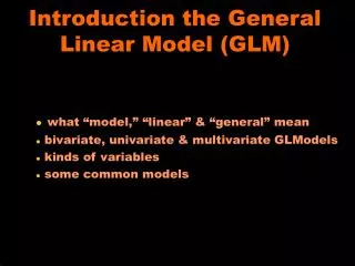
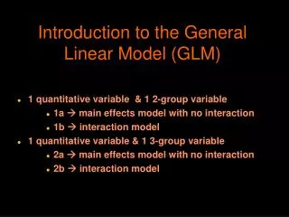
Introduction to the General Linear Model (GLM) • 1 quantitative variable & 1 2-group variable • 1a main effects model with no interaction • 1b interaction model • 1 quantitative variable & 1 3-group variable • 2a main effects model with no interaction • 2b interaction model
There are two important variations of each of these models • Main effects model • Centered or coded terms for each variable • No interaction – assumes regression slope homogeneity • b-weights for binary & quant variables each represent main effect of that variable • 2. Interaction model • Centered or coded terms for each variable • Term for interaction - does not assume reg slp homogen !! • b-weights for binary & quant variables each represent the simple effect of that variable when the other variable = 0 • b-weight for the interaction term represented how the simple effect of one variable changes with changes in the value of the other variable (e.g., the extent and direction of the interaction)
#1a centered quant variable & dummy coded 2-grp variable y’ = b0+ b1x+ b2z “X” is a centered quantitative variable X X – Xmean “Z” is a dummy-coded 2-group variable (Cz = 0 & Tx = 1) Z Tz = 1 Cz = 0
#1a centered quant variable & dummy coded 2-grp variable y’ = b0+ b1x+ b2z • b0 mean of those in Cz with X=0 (mean) • b1 slope of Y-X regression line for Cz (=0) • - slope same for both groups no interaction • b2 group difference for X=mean (=0) • - group different same for all values of X no interaction
#1a quantitative (Xcen) & 2-group (Tz=1 Cz=0) y’ = b0 + b1X + b2Z 20 5 10 b0 = ht of Cz line b1 = slp of Cz line 0 10 20 30 40 50 60 b2 = htdif Cz & Tz Tz Z-lines have same slp (no interaction) Cz -2 -1 0 1 2 Xcen
#1b centered quant var, dummy coded 2-group var & their product term/interaction y’ = b0+ b1x+ b2z+ b3xz “X” is a centered quantitative variable X X – Xmean “Z” is a dummy-coded 2-group variable Z Tz = 1 Cz = 0 “XZ” represents the interaction of “X” and “Z” XZX*Z
#1b centered quant var, dummy coded 2-group var & their product term/interaction y’ = b0+ b1x+ b2z+ b3xz • b0 mean of those in Cz with X= 0 (mean) • b1 slope of Y-X regression line for Cz (=0)* • b2 group difference for X=0 (mean)* • b3 how slope of y-x reg line for Tz (=1) differs from slope of y-x reg line for Cz (=0) • * Because the interaction is included, slopes may be different for different grps • * Because the interaction is included, group differences may be different for different X values
#1b quantitative (X) & 2-group (Tz Cz) predictors w/ interaction y’ = b0 + b1X + b2Z + b3XZ 30 15 15 -5 b0 = ht of Cz line Tz b1 = slp of Cz line b2 = htdif Cz & Tz 0 10 20 30 40 50 60 b3 = slpdif Cz & Tz Cz -2 -1 0 1 2 Xcen
#1b quantitative (X) & 2-group (Tz Cz) predictors w/ interaction y’ = b0 + b1X + b2Z + b3XZ b0 = ht of Cz line b1 = slp of Cz line b2 = htdif Cz & Tz 0 10 20 30 40 50 60 b3 = slpdif Cz & Tz -2 -1 0 1 2 Xcen
#1b quantitative (X) & 2-group (Tz Cz) predictors w/ interaction y’ = b0 + b1X + b2Z + b3XZ b0 = ht of Cz line b1 = slp of Cz line b2 = htdif Cz & Tz 0 10 20 30 40 50 60 b3 = slpdif Cz & Tz -2 -1 0 1 2 Xcen
#1b quantitative (X) & 2-group (Tz Cz) predictors w/ interaction y’ = b0 + b1X + b2Z + b3XZ b0 = ht of Cz line b1 = slp of Cz line b2 = htdif Cz & Tz 0 10 20 30 40 50 60 b3 = slpdif Cz & Tz -2 -1 0 1 2 Xcen
#1b quantitative (X) & 2-group (Tz Cz) predictors w/ interaction y’ = b0 + b1X + b2Z + b3XZ b0 = ht of Cz line b1 = slp of Cz line b2 = htdif Cz & Tz 0 10 20 30 40 50 60 b3 = slpdif Cz & Tz -2 -1 0 1 2 Xcen
#1b quantitative (X) & 2-group (Tz Cz) predictors w/ interaction y’ = b0 + b1X + b2Z + b3XZ b0 = ht of Cz line b1 = slp of Cz line b2 = htdif Cz & Tz 0 10 20 30 40 50 60 b3 = slpdif Cz & Tz -2 -1 0 1 2 Xcen
#1b quantitative (X) & 2-group (Tz Cz) predictors w/ interaction y’ = b0 + b1X + b2Z + b3XZ b0 = ht of Cz line b1 = slp of Cz line b2 = htdif Cz & Tz 0 10 20 30 40 50 60 b3 = slpdif Cz & Tz -2 -1 0 1 2 Xcen
#1b quantitative (X) & 2-group (Tz Cz) predictors w/ interaction y’ = b0 + b1X + b2Z + b3XZ b0 = ht of Cz line b1 = slp of Cz line b2 = htdif Cz & Tz 0 10 20 30 40 50 60 b3 = slpdif Cz & Tz -2 -1 0 1 2 Xcen
#1b quantitative (X) & 2-group (Tz Cz) predictors w/ interaction y’ = b0 + b1X + b2Z + b3XZ b0 = ht of Cz line b1 = slp of Cz line b2 = htdif Cz & Tz 0 10 20 30 40 50 60 b3 = slpdif Cz & Tz -2 -1 0 1 2 Xcen
#1b quantitative (X) & 2-group (Tz Cz) predictors w/ interaction y’ = b0 + b1X + b2Z + b3XZ b0 = ht of Cz line b1 = slp of Cz line b2 = htdif Cz & Tz 0 10 20 30 40 50 60 b3 = slpdif Cz & Tz -2 -1 0 1 2 Xcen
#1b quantitative (X) & 2-group (Tz Cz) predictors w/ interaction y’ = b0 + b1X + b2Z + b3XZ b0 = ht of Cz line b1 = slp of Cz line b2 = htdif Cz & Tz 0 10 20 30 40 50 60 b3 = slpdif Cz & Tz -2 -1 0 1 2 Xcen
#2a centered quant var & dummy coded 3-grp var y’ = b0+ b1x+ b2z1+ b3z2 “X” is centered quantitative variable X X – Xmean “Z1” & “Z2” are dummy-codes for the 3-group variable Z1 Tz1 = 1 Tz2 = 0 Cz = 0 Z2 Tz1 = 0 Tz2 = 1 Cz = 0
#2a centered quant var & dummy coded 3-grp var y’ = b0+ b1x+ b2z1+ b3z2 • b0 mean of those in Cz with X=0 (mean) • b1 slope of Y-X regression line for Cz (=0) • - slope same for all groups no interaction • b2 Tz1 - Cz difference for X=mean (=0) • - group different same for all values of X no interaction • b3 Tz2 - Cz difference for X=mean (=0) • - group different same for all values of X no interaction
#2a quantitative (Xcen) & 3-group Z1 Tz1 = 1 Tz2 = 0 Cz = 0 • Z2 Tz1=0 Tz2 = 1 Cz = 0 y’ = b0 + b1X+ b2Z1 + b3Z2 35 5 5 -15 b0 = ht of Cz line Tz2 b1 = slp of Cz line Cz b2 = htdif Cz & Tz1 0 10 20 30 40 50 60 Tz1 b3 = htdif Cz & Tz2 Z-lines have same slp (no interaction) -2 -1 0 1 2 X
#2b centered quant var, dummy coded 3-group var & their product terms/interaction y’ = b0+ b1x+ b2z1+ b3z2+ b4xz1+ b5xz2 “X” is centered quantitative variable X X – Xmean “Z1” & “Z2” are dummy-codes for the 3-group variable Z1 Tz1 = 1 Tz2 = 0 Cz = 0 Z2 Tz1 = 0 Tz2 = 1 Cz = 0 “XZ1” & “XZ2” represent the interaction of “X” and “Z” XZ1X*Z1 XZ2X*Z2
#2b centered quant var, dummy coded 3-group var & their product terms/interaction y’ = b0+ b1x+ b2z1+ b3z2+ b4xz1+ b5xz2 • b0 mean of those in Cz with X= 0 (mean) • b1 slope of Y-X regression line for Cz • b2 Tz1 - Cz difference for X=0 (mean)* • b3 Tz2 - Cz difference for X=0 (mean)* • b4 how slope of y-x reg line for Tz1 differs from slope of y-x reg line for Cz * • b4 how slope of y-x reg line for Tz2 differs from slope of y-x reg line for Cz * • *Because the interaction is included, group differences may be different for different X values • * Because the interaction is included, slopes may be different for different grps
#2b quantitative (Xcen) & 3-group Z1 Tz1 = 1 Tz2 = 0 Cz = 0 • Z2 Tz1=0 Tz2 = 1 Cz = 0 • and interactions XZ1 = X*Z1 XZ2 = X*Z2 y’ = b0 + b1Xcen + b2Z1 + b3Z2 + b4XZ1 + b5XZ2 -8 2 5 30 15 5 b0 = ht of Cz line b1 = slp of Cz line Tx2 b2 = htdif Cz & Tz1 0 10 20 30 40 50 60 b4 = slpdif Cz & Tz1 Tx1 b3 = htdif Cz & Tz2 Cx b5 = slpdif Cz & Tz2 -2 -1 0 1 2 Xcen
#2b quantitative (Xcen) & 3-group Z1 Tz1 = 1 Tz2 = 0 Cz = 0 • Z2 Tz1=0 Tz2 = 1 Cz = 0 • and interactions XZ1 = X*Z1 XZ2 = X*Z2 y’ = b0 + b1Xcen + b2Z1 + b3Z2 + b4XZ1 + b5XZ2 b0 = ht of Cz line b1 = slp of Cz line b2 = htdif Cz & Tz1 0 10 20 30 40 50 60 b4 = slpdif Cz & Tz1 b3 = htdif Cz & Tz2 b5 = slpdif Cz & Tz2 -2 -1 0 1 2 Xcen
#2b quantitative (Xcen) & 3-group Z1 Tz1 = 1 Tz2 = 0 Cz = 0 • Z2 Tz1=0 Tz2 = 1 Cz = 0 • and interactions XZ1 = X*Z1 XZ2 = X*Z2 y’ = b0 + b1Xcen + b2Z1 + b3Z2 + b4XZ1 + b5XZ2 b0 = ht of Cz line b1 = slp of Cz line b2 = htdif Cz & Tz1 0 10 20 30 40 50 60 b4 = slpdif Cz & Tz1 b3 = htdif Cz & Tz2 b5 = slpdif Cz & Tz2 -2 -1 0 1 2 Xcen
#2b quantitative (Xcen) & 3-group Z1 Tz1 = 1 Tz2 = 0 Cz = 0 • Z2 Tz1=0 Tz2 = 1 Cz = 0 • and interactions XZ1 = X*Z1 XZ2 = X*Z2 y’ = b0 + b1Xcen + b2Z1 + b3Z2 + b4XZ1 + b5XZ2 b0 = ht of Cz line b1 = slp of Cz line b2 = htdif Cz & Tz1 0 10 20 30 40 50 60 b4 = slpdif Cz & Tz1 b3 = htdif Cz & Tz2 b5 = slpdif Cz & Tz2 -2 -1 0 1 2 Xcen
#2b quantitative (Xcen) & 3-group Z1 Tz1 = 1 Tz2 = 0 Cz = 0 • Z2 Tz1=0 Tz2 = 1 Cz = 0 • and interactions XZ1 = X*Z1 XZ2 = X*Z2 y’ = b0 + b1Xcen + b2Z1 + b3Z2 + b4XZ1 + b5XZ2 b0 = ht of Cz line b1 = slp of Cz line b2 = htdif Cz & Tz1 0 10 20 30 40 50 60 b4 = slpdif Cz & Tz1 b3 = htdif Cz & Tz2 b5 = slpdif Cz & Tz2 -2 -1 0 1 2 Xcen
#2b quantitative (Xcen) & 3-group Z1 Tz1 = 1 Tz2 = 0 Cz = 0 • Z2 Tz1=0 Tz2 = 1 Cz = 0 • and interactions XZ1 = X*Z1 XZ2 = X*Z2 y’ = b0 + b1Xcen + b2Z1 + b3Z2 + b4XZ1 + b5XZ2 b0 = ht of Cz line b1 = slp of Cz line b2 = htdif Cz & Tz1 0 10 20 30 40 50 60 b4 = slpdif Cz & Tz1 b3 = htdif Cz & Tz2 b5 = slpdif Cz & Tz2 -2 -1 0 1 2 Xcen
#2b quantitative (Xcen) & 3-group Z1 Tz1 = 1 Tz2 = 0 Cz = 0 • Z2 Tz1=0 Tz2 = 1 Cz = 0 • and interactions XZ1 = X*Z1 XZ2 = X*Z2 y’ = b0 + b1Xcen + b2Z1 + b3Z2 + b4XZ1 + b5XZ2 b0 = ht of Cz line b1 = slp of Cz line b2 = htdif Cz & Tz1 0 10 20 30 40 50 60 b4 = slpdif Cz & Tz1 b3 = htdif Cz & Tz2 b5 = slpdif Cz & Tz2 -2 -1 0 1 2 Xcen
#2b quantitative (Xcen) & 3-group Z1 Tz1 = 1 Tz2 = 0 Cz = 0 • Z2 Tz1=0 Tz2 = 1 Cz = 0 • and interactions XZ1 = X*Z1 XZ2 = X*Z2 y’ = b0 + b1Xcen + b2Z1 + b3Z2 + b4XZ1 + b5XZ2 b0 = ht of Cz line b1 = slp of Cz line b2 = htdif Cz & Tz1 0 10 20 30 40 50 60 b4 = slpdif Cz & Tz1 b3 = htdif Cz & Tz2 b5 = slpdif Cz & Tz2 -2 -1 0 1 2 Xcen
#2b quantitative (Xcen) & 3-group Z1 Tz1 = 1 Tz2 = 0 Cz = 0 • Z2 Tz1=0 Tz2 = 1 Cz = 0 • and interactions XZ1 = X*Z1 XZ2 = X*Z2 y’ = b0 + b1Xcen + b2Z1 + b3Z2 + b4XZ1 + b5XZ2 b0 = ht of Cz line b1 = slp of Cz line b2 = htdif Cz & Tz1 0 10 20 30 40 50 60 b4 = slpdif Cz & Tz1 b3 = htdif Cz & Tz2 b5 = slpdif Cz & Tz2 -2 -1 0 1 2 Xcen
#2b quantitative (Xcen) & 3-group Z1 Tz1 = 1 Tz2 = 0 Cz = 0 • Z2 Tz1=0 Tz2 = 1 Cz = 0 • and interactions XZ1 = X*Z1 XZ2 = X*Z2 y’ = b0 + b1Xcen + b2Z1 + b3Z2 + b4XZ1 + b5XZ2 b0 = ht of Cz line b1 = slp of Cz line b2 = htdif Cz & Tz1 0 10 20 30 40 50 60 b4 = slpdif Cz & Tz1 b3 = htdif Cz & Tz2 b5 = slpdif Cz & Tz2 -2 -1 0 1 2 Xcen
#2b quantitative (Xcen) & 3-group Z1 Tz1 = 1 Tz2 = 0 Cz = 0 • Z2 Tz1=0 Tz2 = 1 Cz = 0 • and interactions XZ1 = X*Z1 XZ2 = X*Z2 y’ = b0 + b1Xcen + b2Z1 + b3Z2 + b4XZ1 + b5XZ2 b0 = ht of Cz line b1 = slp of Cz line b2 = htdif Cz & Tz1 0 10 20 30 40 50 60 b4 = slpdif Cz & Tz1 b3 = htdif Cz & Tz2 b5 = slpdif Cz & Tz2 -2 -1 0 1 2 Xcen