Introduction: The General Linear Model
Introduction: The General Linear Model. The General Linear Model is a phrase used to indicate a class of statistical models which include simple linear regression analysis. Regression is the predominant statistical tool used in the social sciences due to its simplicity and versatility.

Introduction: The General Linear Model
E N D
Presentation Transcript
Introduction: The General Linear Model • The General Linear Model is a phrase used to indicate a class of statistical models which include simple linear regression analysis. • Regression is the predominant statistical tool used in the social sciences due to its simplicity and versatility. • Also called Linear Regression Analysis.
Simple Linear Regression: The Basic Mathematical Model • Regression is based on the concept of the simple proportional relationship - also known as the straight line. • We can express this idea mathematically! • Theoretical aside: All theoretical statements of relationship imply a mathematical theoretical structure. • Just because it isn’t explicitly stated doesn’t mean that the math isn’t implicit in the language itself!
Simple Linear Relationships • Alternate Mathematical Notation for the straight line - don’t ask why! • 10th Grade Geometry • Statistics Literature • Econometrics Literature
Alternate Mathematical Notation for the Line • These are all equivalent. We simply have to live with this inconsistency. • We won’t use the geometric tradition, and so you just need to remember that B0 and a are both the same thing.
Linear Regression: the Linguistic Interpretation • In general terms, the linear model states that the dependent variable is directly proportional to the value of the independent variable. • Thus if we state that some variable Y increases in direct proportion to some increase in X, we are stating a specific mathematical model of behavior - the linear model.
The Mathematical Interpretation: The Meaning of the Regression Parameters • a = the intercept • the point where the line crosses the Y-axis. • (the value of the dependent variable when all of the independent variables = 0) • b = the slope • the increase in the dependent variable per unit change in the independent variable (also known as the 'rise over the run')
The Error Term • Such models do not predict behavior perfectly. • So we must add a component to adjust or compensate for the errors in prediction. • Having fully described the linear model, the rest of the semester (as well as several more) will be spent of the error.
The Nature of Least Squares Estimation • There is 1 essential goal and there are 4 important concerns with any OLS Model
The 'Goal' of Ordinary Least Squares • Ordinary Least Squares (OLS) is a method of finding the linear model which minimizes the sum of the squared errors. • Such a model provides the best explanation/prediction of the data.
Why Least Squared error? • Why not simply minimum error? • The error’s about the line sum to 0.0! • Minimum absolute deviation (error) models now exist, but they are mathematically cumbersome. • Try algebra with | Absolute Value | signs!
Other models are possible... • Best parabola...? • (i.e. nonlinear or curvilinear relationships) • Best maximum likelihood model ... ? • Best expert system...? • Complex Systems…? • Chaos models • Catastrophe models • others
The Simple Linear Virtue • I think we over emphasize the linear model. • It does, however, embody this rather important notion that Y is proportional to X. • We can state such relationships in simple English. • As unemployment increases, so does the crime rate.
The Notion of Linear Change • The linear aspect means that the same amount of increase unemployment will have the same effect on crime at both low and high unemployment. • A nonlinear change would mean that as unemployment increased, its impact upon the crime rate might increase at higher unemployment levels.
Why squared error? • Because: • (1) the sum of the errors expressed as deviations would be zero as it is with standard deviations, and • (2) some feel that big errors should be more influential than small errors. • Therefore, we wish to find the values of a and b that produce the smallest sum of squared errors.
Minimizing the Sum of Squared Errors • Who put the Least in OLS • In mathematical jargon we seek to minimize the Unexplained Sum of Squares (USS), where:
The Parameter estimates • In order to do this, we must find parameter estimates which accomplish this minimization. • In calculus, if you wish to know when a function is at its minimum, you take the first derivative. • In this case we must take partial derivatives since we have two parameters (a & b) to worry about. • We will look closer at this and it’s not a pretty sight!
Why squared error? • Because • (1) the sum of the errors expressed as deviations would be zero as it is with standard deviations, and • (2) some feel that big errors should be more influential than small errors. • Therefore, we wish to find the values of a and b that produce the smallest sum of squared errors.
Sum of Squares Terminology • In mathematical jargon we seek to minimize the Unexplained Sum of Squares (USS), where:
The Parameter estimates • In order to do this, we must find parameter estimates which accomplish this minimization. • In calculus, if you wish to know when a function is at its minimum, you take the first derivative. • In this case we must take partial derivatives since we have two parameters to worry about.
Tests of Inference • t-tests for coefficients • F-test for entire model
T-Tests • Since we wish to make probability statements about our model, we must do tests of inference. • Fortunately,
Goodness of Fit • Since we are interested in how well the model performs at reducing error, we need to develop a means of assessing that error reduction. Since the mean of the dependent variable represents a good benchmark for comparing predictions, we calculate the improvement in the prediction of Yi relative to the mean of Y (the best guess of Y with no other information).
Sums of Squares • This gives us the following 'sum-of-squares' measures: • Total Variation = Explained Variation + Unexplained Variation
Sums of Squares Confusion • Note: Occasionally you will run across ESS and RSS which generate confusion since they can be used interchangeably. ESS can be error sums-of-squares or estimated or explained SSQ. Likewise RSS can be residual SSQ or regression SSQ. Hence the use of USS for Unexplained SSQ in this treatment.
Measures of Goodness of fit • The Correlation coefficient • r-squared
The correlation coefficient • A measure of how close the residuals are to the regression line • It ranges between -1.0 and +1.0 • It is closely related to the slope.
R2 (r-square) • The r2 (or R-square) is also called the coefficient of determination.
Tests of Inference • t-tests for coefficients • F-test for entire modelSince we are interested in how well the model performs at reducing error, we need to develop a means of assessing that error reduction. Since the mean of the dependent variable represents a good benchmark for comparing predictions, we calculate the improvement in the prediction of Yi relative to the mean of Y (the best guess of Y with no other information).This gives us the following 'sums-of-squares' measures:
Goodness of fit • The correlation coefficient • A measure of how close the residuals are to the regression lineIt ranges between -1.0 and +1.0 • r2 (r-square) • The r-square (or R-square) is also called the coefficient of determination
Extra Material on OLS: The Adjusted R2 • Since R2 always increases with the addition of a new variable, the adjusted R2 compensates for added explanatory variables.
Extra Material on OLS: The F-test • In addition, the F test for the entire model must be adjusted to compensate for the changed degrees of freedom. • Note that F increases as n or R2 increases and decreases as k increasesAdding a variable will always increase R2, but not necessarily adjusted R2 or F. In addition values of R2 below 0.0 are possible.