General Linear Model
General Linear Model. Beatriz Calvo Davina Bristow. Overview. Summary of regression Matrix formulation of multiple regression Introduce GLM Parameter Estimation Residual sum of squares GLM and fMRI fMRI model Linear Time Series Design Matrix Parameter estimation Summary.


General Linear Model
E N D
Presentation Transcript
General Linear Model Beatriz Calvo Davina Bristow
Overview • Summary of regression • Matrix formulation of multiple regression • Introduce GLM • Parameter Estimation • Residual sum of squares • GLM and fMRI • fMRI model • Linear Time Series • Design Matrix • Parameter estimation • Summary
Summary of Regression • Linear regression models the linear relationship between a single dependent variable, Y, and a single independent variable, X, using the equation: Y = βX + c + ε • The regression coefficient, β, reflects how much of an effect X has on Y • ε is the error term and is assumed to be independently, identically, and normally distributed (mean 0 and variance σ2)
Summary of Regression • Multiple regression is used to determine the effect of a number of independent variables, X1, X2, X3 etc, on a single dependent variable, Y • The different X variables are combined in a linear way and each has its own regression coefficient: Y = β1X1 + β2X2 +…..+ βLXL + ε • The β parameters reflect the independent contribution of each independent variable, X, to the value of the dependent variable, Y. • i.e. the amount of variance in Y that is accounted for by each X variable after all the other X variables have been accounted for
Matrix formulation • Multiplying matrices reminder: G H I G x a + H x b + I x c G x d + H x e + I x f a b c d e f x =
Matrix Formulation • Write out equation for each observation of variable Y from 1 to J: Y1 = X11β1 +…+X1lβl +…+X1LβL + ε1 Yj = Xj1β1 +…+Xjlβl +…+ XjLβL + εj YJ = XJ1β1 +…+XJlβl +…+ XJLβL + εJ • Can turn these simultaneous equations into matrix form to get a single equation: β1 βj βJ ε1 εj εJ Y1 Yj YJ X11 … X1l … X1L Xj1 … X1l… X1L X11 … X1l… X1L + = Y = X x β + ε Design Matrix Parameters Residuals/Error Observed data
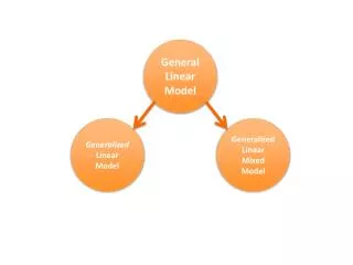
General Linear Model • This is simply an extension of multiple regression • Or alternatively Multiple Regression is just a simple form of the General Linear Model • Multiple Regression only looks at ONE dependent (Y) variable • Whereas, GLM allows you to analyse several dependent, Y, variables in a linear combination • i.e. multiple regression is a GLM with only one Y variable • ANOVA, t-test, F-test, etc. are also forms of the GLM
GLM - continued.. • In the GLM the vector Y, of J observations of a single Y variable, becomes a MATRIX, of J observations of N different Y variables • An fMRI experiment could be modelled with matrix Y of the BOLD signal at N voxels for J scans • However SPM takes a univariate approach, i.e. each voxel is represented by a column vector of J fMRI signal measurements, and it processed through a GLM separately • (this is why you then need to correct for multiple comparisons)
GLM and fMRI How does the GLM apply to fMRI experiments? Y= X. β+ ε Observed data: SPM uses a mass univariate approach – that is each voxel is treated as a separate column vector of data. Y is the BOLD signal at various time points at a single voxel Design matrix: Several components which explain the observed data, i.e. the BOLD time series for the voxel Timing info: onset vectors, Omj, and duration vectors, Dmj HRF, hm, describes shape of the expected BOLD response over time Other regressors, e.g. realignment parameters Parameters: Define the contribution of each component of the design matrix to the value of Y Estimated so as to minimise the error, ε, i.e. least sums of squares Error: Difference between the observed data, Y, and that predicted by the model, Xβ. Not assumed to be spherical in fMRI
Parameter estimation • In linear regression the parameter β is estimated so that the best prediction of Y can be obtained from X • i.e. sums of squares of difference between predicted values and observed data, (i.e. the residuals, ε) is minimised • Remember last week’s talk & graph! • The method of estimating parameters in GLM is essentially the same, i.e. minimising sums of squares (ordinary least squares), it just looks more complicated
Last week’s graph ε = ỹ , predicted value = y i , true value ε = residual error y = βx + c
Residual Sums of Squares • Take a set of parameter estimates, β • Put these into the GLM equation to obtain estimates of Y from X, i.e. fitted values, Y: Y = X x β • The residual errors, e, are the difference between the fitted and actual values: e = Y - Y = Y - Xβ • Residual sums of squares is: S = ΣjJej2 • When written out in full this gives: S = ΣjJ(Yj- Xj1β1 -…- XjLβL)2
Minimising S e = Y - Xβ S = ΣjJej2 • If you plot the sum of squares value for different parameter, β, estimates you get a curve S = Σ(Y - Xβ)2 • S is minimised when the gradient of this curve is zero Gradient = 0 min S
Minimising S cont. • so to calculate the values of β which gives you the least sums of squares you must find the partial derivative of S = ΣjJ(Yj- Xj1β1 -…- XjLβL)2 • Which is ∂S/∂β = 2Σ(-Xjl)(Yj – Xj1β1-…- XjLβL) and solve this for ∂S/∂β = 0 • In matrix form of the residual sum of squares is S = eTe this is equivalent to ΣjJej2 (remember how we multiply matrices) • e = Y - Xβtherefore S = (Y - Xβ )T(Y - Xβ )
Minimising S cont. • Need to find the derivative and solve for ∂S/∂β = 0 • The derivative of this equation can be rearranged to give XTY = (XTX)β when the gradient of the curve = 0, i.e. S is minimised • This can be rearranged to give: β = XTY(XTX)-1 • But a solution can only be found, if (XTX) is invertible because you need to divide by it, which in matrix terms is the same as multiplying by the inverse!
GLM and fMRI How does the GLM apply to fMRI experiments? Y= X. β+ ε Observed data: SPM uses a mass univariate approach – that is each voxel is treated as a separate column vector of data. Y is the BOLD signal at various time points at a single voxel Design matrix: Several components which explain the observed data, i.e. the BOLD time series for the voxel Timing info: onset vectors, Omj, and duration vectors, Dmj HRF, hm, describes shape of the expected BOLD response over time Other regressors, e.g. realignment parameters Parameters: Define the contribution of each component of the design matrix to the value of Y Estimated so as to minimise the error, ε, i.e. least sums of squares Error: Difference between the observed data, Y, and that predicted by the model, Xβ. Not assumed to be spherical in fMRI
fMRI models • Completed the experiment, after preprocessing, the data are ready for STATS. • STATS: (estimate parameters, β, inference) • indicating evidence against the Ho of no effect at each voxel are computed->an image of this statistic is produce • This statistical image is assessed (other talk will explain that)
Example: 1 subject. 1 session Each epoch 6 scans Whole brain acquisition data Moving finger vs rest 7 cycles of rest and moving Time series of BOLD response in one voxel Question: Is there any change in the BOLD response between moving and rest? Responses at voxel (x, y, z) Timeseconds
Time Linear Time Series Model • TIME SERIES: consist on the sequential measures of fMRI data signal intensities over the period of the experiment • The same temporal model is used at each voxel • Mass-univariated model and perform the same analysis at each voxel • Therefore, we can describe the complete temporal model for fMRI data by looking at how it works for the data from a voxel. Single Voxel Time Series
Y: My data/ observations My Data • Time series of N observations Y1,…,Ys,…,Yn. N= scan number • Acquired at one voxel at times ts, where S=1:N Time Y1 Ys YN Single Voxel Time Series
Model specification • The overall aim of regressor generation is to come up with a design matrix that models the expected fMRI response at any voxel as a linear combinations of columns. • Design matrix – formed of several components which explain the observed data. • Two things SPM need to know to construct the design matrix: • Specify regressors • Basis functions that explain my data
Model specification … • Specify regressors X • Timing information consists of onset vectors Omj and duration vectors Dm • Other regressors e.g. movement parameters • Include as many regressors as you consider necessary to best explain what’s going on. • Basis functions that explain my data (HRF) • Expected shape of the BOLD response due to stimulus presentation
GLM and fMRI data • Model the observed time series at each voxel as a linear combination of explanatory functions, plus an error term Ys= β1X1(tS)+ …+ βlXl(tS)+ …+ βLXL(tS) + εs • Here, each column of the design matrix X contains the values of one of the continuous regressors evaluated at each time point ts of fMRI time series • That is, the columns of the design matrix are the discrete regressors
GLM and fMRI data … • Consider the equation for all time points, to give a set of equations Y1= β1X1(t1)+ …+ βlXl(t1)+ …+ βLXL(t1) + ε1 Ys= β1 X1(tS)+ …+ βl Xl(tS)+ …+ βLXL(tS)+ εs YN= β1X1(tN)+ …+ βlXl(tN)+ …+ βLXL(tN) + εN In matrix form: X1(t1)Xl(t1) XL(t1) X1(tS) Xl(tS) XL(tS) X1(tN) Xl(tN) XL(tN) β1 βl βL εN εs εN Y1 Ys YN = + Y = Xβ + ε In matrix notation:
Getting the design matrix Observations Regressors β1 ε Errors are normally and independently and identical distributed β2 = + + Time Intensity y = x1x2
Getting the design matrix … Observations Regressors Error β2 β1 + + = Time Intensity y = β1x1 + β2x2 + ε
Design matrix Observations Regressors Error β1 x + = β2 Y = X β + ε
εN εs εN Y1 Ys YN X1(t1)Xl(t1) XL(t1) X1(tS) Xl(tS) XL(tS) X1(tN) Xl(tN) XL(tN) β1 βl βL Design matrix Observations Regressors Error L l l l • Model is specified by: • design matrix • Assumptions about ε β2 Y = Xβ + ε β1 L N N N N: nuber of scans P: number of regressors Y = Xβ + ε
Parametric estimation ε = Y - Y = Y - Xβ β2 = + S = ΣtJεt2 + β1 The error is minimal when β= XTY(XTX)-1 Least squares Parameter estimates YXε Estimate parameters β (Get this by putting into matrix form and finding derivative)
Summary • The General Linear Model allows you to find the parameters, β, which provide the best fit with your data, Y • The optimal parameters estimates, β, are found by minimising the Sums of Squares differences between your predicted model and the observed data • The design matrix in SPM contains the information about the factors, X, which may explain the observed data • Once we have obtained the βs at each voxel we can use these to do various statistical tests but that is another talk….
THE END Thank you to Lucy, Daniel and Will and to Stephan for his chapter and slides about GLM and to Adam for last year’s presentation Links: http://www.fil.ion.ucl.ac.uk/~wpenny/notes03/slides/glm/slide1.htm http://www.fil.ion.ucl.ac.uk/spm/HBF2/pdfs/Ch7.pdf http://www.fil.ion.ucl.ac.uk/~wpenny/mfd/GLM.ppt