The General Linear Model
The General Linear Model. The Simple Linear Model. Linear Regression. Suppose that we have two variables. Y – the dependent variable (response variable) X – the independent variable (explanatory variable, factor). X , the independent variable may or may not be a random variable.


The General Linear Model
E N D
Presentation Transcript
The Simple Linear Model Linear Regression
Suppose that we have two variables • Y – the dependent variable (response variable) • X – the independent variable (explanatory variable, factor)
X , the independent variable may or may not be a random variable . Sometimes it is randomly observed. Sometimes specific values of X are selected
The dependent variable, Y, is assumed to be a random variable . The distribution of Y is dependent on X The object is to determine that distribution using statistical techniques. (Estimation and Hypothesis Testing)
These decisions will be based on data collected on both variable Y (the dependent variable) and X (the independent variable) . Let (x1, y1), (x2, y2), … ,(xn, yn) denote n pairs of values measured on the independent variable (X) and the dependent variable (Y) The scatterplot: The graphical plot of the points: (x1, y1), (x2, y2), … ,(xn, yn)
Assume that we have collected data on two variables X and Y. Let (x1, y1) (x2, y2) (x3, y3) … (xn, yn) denote thepairs of measurements on the on two variables X and Y for n cases in a sample (or population)
The assumption will be made that y1,y2, y3 …, yn are • independent random variables. • Normally distributed. • Have the common variance, s. • The mean of yiis mi = a+ bxi Data that satisfies the assumptions above is to come from the Simple Linear Model
Each yi is assumed to be randomly generated from a normal distribution with mean mi = a + bxi and standard deviation s. yi s a + bxi xi
When data is correlated it falls roughly about a straight line.
The density of yi is: The joint density of y1,y2, …,yn is:
Estimation of the parameters the intercept a the slope b the standard deviation s (or variance s2)
The Least Squares Line Fitting the best straight line to “linear” data
Let Y = a + b X denote an arbitrary equation of a straight line. a and b are known values. This equation can be used to predict for each value of X, the value of Y. For example, if X = xi (as for the ith case) then the predicted value of Y is:
Define the residual for each case in the sample to be: The residual sum of squares (RSS) is defined as: The residual sum of squares (RSS) is a measure of the “goodness of fit of the line Y = a + bX to the data
One choice of a and b will result in the residual sum of squares attaining a minimum. If this is the case than the line: Y = a + bX is called the Least Squares Line
To find the Least Squares estimates, a and b, we need to solve the equations: and
Note: or and
Note: or
and Hence the optimal values of a and b satisfy the equations: From the first equation we have: The second equation becomes:
Solving the second equation for b: and where and
and Note: Proof
Summary: Slope and intercept of the least squares Line and
Maximum Likelihood Estimation of the parameters the intercept a the slope b the standard deviation s
Recall The joint density of y1,y2, …,yn is: = the Likelihood function
the log Likelihood function To find the maximum Likelihood estimates of a,band swe need to solve the equations:
becomes becomes These are the same equations for the least squares line which have solution:
The third equation: becomes
and A computing formula for the estimate of s2 Hence
Now Hence
It also can be shown that Thus , the maximum likelihood estimator of s2, is a biased estimator of s2. This estimator can be easily converted into an unbiased estimator of s2 by multiply by the ratio n/(n – 2)
Application Of Statistical Theory to simple Linear Regression We will now use statistical theory to prove optimal properties of the estimators. Recall, the joint density of y1,y2, …,yn is:
Also and Thus all three estimators are functions of the set of complete sufficient statistics. If they are also unbiased then they are Uniform Minimum Variance Unbiased (UMVU) estimators (using the Lehmann-Scheffe theorem)
We have already shown that s2 is an unbiased estimator of s2. We need only show that: and are unbiased estimators of band a.
Thus are unbiased estimators of band a.
Also Thus
Consider the random variable Y with 1. E[Y] = b1X1+ b2X2 + ... + bpXp (alternatively E[Y] = b0+b1X1+ ... + bpXp, intercept included) and 2. var(Y) = s2 • where b1, b2 , ... ,bp are unknown parameters • and X1 ,X2 , ... , Xp are nonrandom variables. • Assume further that Y is normally distributed.
Thus the density of Y is: f(Y|b1, b2 , ... ,bp, s2) = f(Y| , s2)
Now suppose that n independent observations of Y, (y1, y2, ..., yn) are made corresponding to n sets of values of (X1 ,X2 , ... , Xp) - (x11 ,x12 , ... , x1p), (x21 ,x22 , ... , x2p), ... (xn1 ,xn2 , ... , xnp). Then the joint density of y = (y1, y2, ... yn) is: f(y1, y2, ..., yn|b1, b2 , ... ,bp, s2) =
Thus is a member of the exponential family of distributions And is a Minimal Complete set of Sufficient Statistics.
Matrix-vector formulation The General Linear Model