Download
1 / 31
310 likes | 444 Vues
This document provides a comprehensive overview of the General Linear Model (GLM) applied to fMRI data analysis, particularly within the field of neuroeconomics. It discusses the structure and assumptions of the design matrix, parameter estimation via ordinary least squares, and the challenges associated with BOLD response modeling, including issues with low-frequency noise and temporal autocorrelation. Additionally, solutions such as convolution modeling of the hemodynamic response function (HRF) and high-pass filtering techniques are explored, enhancing the accuracy of statistical parametric mapping (SPM) analysis.

E N D
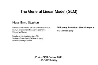
The General Linear Model (GLM) Klaas Enno Stephan Laboratory for Social & Neural Systems Research Institute for Empirical Research in Economics University of Zurich Functional Imaging Laboratory (FIL) Wellcome Trust Centre for Neuroimaging University College London With many thanks for slides & images to: FIL Methods group Methods & models for fMRI data analysis in neuroeconomicsNovember 2010
Overview of SPM Statistical parametric map (SPM) Design matrix Image time-series Kernel Realignment Smoothing General linear model Gaussian field theory Statistical inference Normalisation p <0.05 Template Parameter estimates
A very simple fMRI experiment One session Passive word listening versus rest 7 cycles of rest and listening Blocks of 6 scans with 7 sec TR Stimulus function Question: Is there a change in the BOLD response between listening and rest?
Modelling the measured data Why? Make inferences about effects of interest • Decompose data into effects and error • Form statistic using estimates of effects and error How? stimulus function effects estimate linear model statistic data error estimate
model specification parameter estimation hypothesis statistic Voxel-wise time series analysis Time Time BOLD signal single voxel time series SPM
Single voxel regression model error = + + 1 2 Time e x1 x2 BOLD signal
Mass-univariate analysis: voxel-wise GLM X + y = • Model is specified by • Design matrix X • Assumptions about e N: number of scans p: number of regressors The design matrix embodies all available knowledge about experimentally controlled factors and potential confounds.
GLM assumes Gaussian “spherical” (i.i.d.) errors Examples for non-sphericity: sphericity = i.i.d.error covariance is scalar multiple of identity matrix: Cov(e) = 2I non-identity non-independence
Parameter estimation Objective: estimate parameters to minimize = + X y Ordinary least squares estimation (OLS) (assuming i.i.d. error):
A geometric perspective on the GLM Residual forming matrix R OLS estimates y e x2 x1 Projection matrix P Design space defined by X
Deriving the OLS equation OLS estimate
Correlated and orthogonal regressors y x2 x2* x1 Correlated regressors = explained variance is shared between regressors When x2 is orthogonalized with regard to x1, only the parameter estimate for x1 changes, not that for x2!
HRF What are the problems of this model? • BOLD responses have a delayed and dispersed form. • The BOLD signal includes substantial amounts of low-frequency noise. • The data are serially correlated (temporally autocorrelated) this violates the assumptions of the noise model in the GLM
hemodynamic response function (HRF) Problem 1: Shape of BOLD responseSolution: Convolution model The response of a linear time-invariant (LTI) system is the convolution of the input with the system's response to an impulse (delta function). expected BOLD response = input function impulse response function (HRF)
Convolution model of the BOLD response Convolve stimulus function with a canonical hemodynamic response function (HRF): HRF
Problem 2: Low-frequency noise Solution: High pass filtering S = residual forming matrix of DCT set discrete cosine transform (DCT) set
blue= data black = mean + low-frequency drift green= predicted response, taking into account low-frequency drift red= predicted response, NOT taking into account low-frequency drift High pass filtering: example
Problem 3: Serial correlations with 1st order autoregressive process: AR(1) autocovariance function
Dealing with serial correlations • Pre-colouring: impose some known autocorrelation structure on the data (filtering with matrix W) and use Satterthwaite correction for df’s. • Pre-whitening: 1. Use an enhanced noise model with multiple error covariance components, i.e. e ~ N(0,2V) instead of e ~ N(0,2I).2. Use estimated serial correlation to specify filter matrix W for whitening the data.
How do we define W ? • Enhanced noise model • Remember linear transform for Gaussians • Choose W such that error covariance becomes spherical • Conclusion: W is a simple function of V so how do we estimate V ?
Estimating V: Multiple covariance components enhanced noise model error covariance components Q and hyperparameters V Q2 Q1 1 + 2 = Estimation of hyperparameters with ReML (restricted maximum likelihood).
Contrasts &statistical parametric maps c = 1 0 0 0 0 0 0 0 0 0 0 Q: activation during listening ? Null hypothesis:
t-statistic based on ML estimates c = 1 0 0 0 0 0 0 0 0 0 0 For brevity: ReML-estimates
Physiological confounds • head movements • arterial pulsations (particularly bad in brain stem) • breathing • eye blinks (visual cortex) • adaptation effects, fatigue, fluctuations in concentration, etc.
Outlook: further challenges • correction for multiple comparisons • variability in the HRF across voxels • slice timing • limitations of frequentist statistics Bayesian analyses • GLM ignores interactions among voxels models of effective connectivity • These issues are discussed in future lectures.
Correction for multiple comparisons • Mass-univariate approach: We apply the GLM to each of a huge number of voxels (usually > 100,000). • Threshold of p<0.05 more than 5000 voxels significant by chance! • Massive problem with multiple comparisons! • Solution: Gaussian random field theory
Variability in the HRF • HRF varies substantially across voxels and subjects • For example, latency can differ by ± 1 second • Solution: use multiple basis functions • See talk on event-related fMRI
Summary • Mass-univariate approach: same GLM for each voxel • GLM includes all known experimental effects and confounds • Convolution with a canonical HRF • High-pass filtering to account for low-frequency drifts • Estimation of multiple variance components (e.g. to account for serial correlations)
Bibliography • Friston, Ashburner, Kiebel, Nichols, Penny (2007) Statistical Parametric Mapping: The Analysis of Functional Brain Images. Elsevier. • Christensen R (1996) Plane Answers to Complex Questions: The Theory of Linear Models. Springer. • Friston KJ et al. (1995) Statistical parametric maps in functional imaging: a general linear approach. Human Brain Mapping 2: 189-210.
Convolution step-by-step (from Wikipedia): • Express each function in terms of a dummy variable τ. • 2. Reflect one of the functions: g(τ)→g( − τ). • 3. Add a time-offset, t, which allows g(t − τ) to slide along the τ-axis. 4.Start t at -∞ and slide it all the way to +∞. Wherever the two functions intersect, find the integral of their product. In other words, compute a sliding, weighted-average of function f(τ), where the weighting function is g( − τ). The resulting waveform (not shown here) is the convolution of functions f and g. If f(t) is a unit impulse, the result of this process is simply g(t), which is therefore called the impulse response.