Understanding General Linear Model in Data Analysis
Explore the basics of General Linear Model in statistical analysis, including regressors, parameters, residuals, and design matrices. Learn about the assumptions, errors, and solutions in GLM using Ordinary Least Squares, with practical examples and references provided.

Understanding General Linear Model in Data Analysis
E N D
Presentation Transcript
General Linear Model regressors β1 β2 . . . βL ε1 ε2 . . . εJ Y1 Y2 . . . YJ X11 … X1l … X1L X21… X2l… X2L . . . XJ1 … XJl… XJL = + time points time points time points regressors Y = X *β + ε Design Matrix Observed data Parameters Residuals/Error
Design Matrix 0 0 0 0 0 0 0 rest task Conditions On Off Off On 1 1 1 1 1 1 1 Use ‘dummy codes’ to label different levels of an experimental factor (eg. On = 1, Off = 0). time
Design Matrix 5 4 4 2 3 1 6 3 1 6 5 2 Covariates Parametric variation of a single variable (eg. Task difficulty = 1-6) or measured values of a variable (eg. Movement).
Design Matrix 1 1 1 1 1 1 1 1 . . . Constant Variable Models the baseline activity (eg. Always = 1)
Design Matrix Time Regressors The design matrix should include everything that might explain the data.
General Linear Model regressors β1 β2 . . . βL ε1 ε2 . . . εJ Y1 Y2 . . . YJ X11 … X1l … X1L X21… X2l… X2L . . . XJ1 … XJl… XJL = + time points time points time points regressors Y = X *β + ε Design Matrix Observed data Parameters Residuals/Error
Error • Independent and identically distributed iid
Ordinary Least Squares Residual sum of square: The sum of the square difference between actual value and fitted value. e
Ordinary Least Squares N å 2 e = minimum t = t 1 e
Ordinary Least Squares Y = Xβ+e e = Y-Xβ XTe=0 => XT(Y-Xβ)=0 => XTY-XTXβ=0 => XTXβ=XTY => β=(XTX)-1XTY y e Xβ x1β1 x2β2
fMRI Y = X *β + ε Observed data Design Matrix Parameters Residuals/Error
The Convolution Model Expected BOLD HRF Impulses =
Convolve stimulus function with a canonical hemodynamic response function (HRF): OriginalConvolvedHRF HRF
Noise Low-frequency noise Solution: High pass filtering
blue= data black = mean + low-frequency drift green= predicted response, taking into account low-frequency drift red= predicted response, NOT taking into account low-frequency drift discrete cosine transform (DCT) set
Assumptions of GLM using OLS All About Error
Unbiasedness Expected value of beta = beta
Autoregressive Model y = Xβ + e overtime et= aet-1 + ε autocovariance function a should = 0
Thanks to… • Dr. Guillaume Flandin
References • http://www.fil.ion.ucl.ac.uk/spm/doc/books/hbf2/pdfs/Ch7.pdf • http://www.fil.ion.ucl.ac.uk/spm/course/slides10-vancouver/02_General_Linear_Model.pdf • Previous MfD presentations