Signal Conditioning and Linearization of RTD Sensors
Signal Conditioning and Linearization of RTD Sensors. 9/24/11. Contents. RTD Overview RTD Nonlinearity Analog Linearization Digital Acquisition and Linearization. What is an RTD?. R esistive T emperature D etector Sensor with a predictable resistance vs. temperature

Signal Conditioning and Linearization of RTD Sensors
E N D
Presentation Transcript
Signal Conditioning and Linearization of RTD Sensors 9/24/11
Contents • RTD Overview • RTD Nonlinearity • Analog Linearization • Digital Acquisition and Linearization
What is an RTD? • Resistive Temperature Detector • Sensor with a predictable resistance vs. temperature • Measure the resistance and calculate temperature based on the Resistance vs. Temperature characteristics of the RTD material PT100 α = 0.00385
How does an RTD work? • L = Wire Length • A = Wire Area • e = Electron Charge (1.6e-19 Coulombs) • n = Electron Density • u = Electron Mobility • The product n*u decreases over temperature, therefore resistance increases over temperature (PTC) • Linear Model of Conductor Resistivity Change vs. Temperature
What is an RTD made of? • Platinum (pt) • Nickel (Ni) • Copper (Cu) • Have relatively linear change in resistance over temp • Have high resistivity allowing for smaller dimensions • Either Thin-Film or Wire-Wound *Images from RDF Corp
How Accurate is an RTD? • Absolute accuracy is “Class” dependant - defined by DIN-IEC 60751. Allows for easy interchangeability of field sensors • Repeatability usually very good, allows for individual sensor calibration • Long-Term Drift usually <0.1C/year, can get as low as 0.0025C/year *AAA (1/10DIN) is not included in the DIN-IEC-60751 spec but is an industry accepted tolerance class for high-performance measurements **Manufacturers may choose to guarantee operation over a wider temperature range than the DIN-IEC60751 provides
Why use an RTD? Table Comparing Advantages and Disadvantages of Temp Sensors
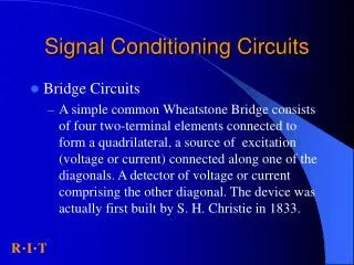
How to Measure an RTD Resistance? • Use a……. Current Source or Wheatstone Bridge
RTD Types and Their Parasitic Lead Resistances 3-Wire 2-Wire 2-Wire with Compensating Loop 4-Wire
3-Wire Measurements Error = 0 as long as Isource1 = Isource2 and RL are equal
4-Wire Measurements System Errors reduced to measurement circuit accuracy
Self-Heating Errors of RTD • Typically 2.5mW/C – 60mW/C • Set excitation level so self-heating error is <10% of the total error budget
RTD Resistance vs Temperature Callendar-Van Dusen Equations Equation Constants for IEC 60751 PT-100 RTD (α = 0.00385)
RTD Nonlinearity Linear fit between the two end-points shows the Full-Scale nonlinearity Nonlinearity = 4.5% Temperature Error > 45C
RTD Nonlinearity B and C terms are negative so 2nd and 3rd order effects decrease the sensor output over the sensor span.
Correcting for Non-Linearity Sensor output decreases over span? Compensate by increasing excitation over span!
Analog Linearization Circuits Two-Wire Single Op-Amp Example Amplifiers: Low-Voltage: OPA333OPA376 High Voltage:OPA188OPA277 This circuit is designed for a 0-5V output for a 0-200C temperature span. Components R2, R3, R4, and R5 are adjusted to change the desired measurement temperature span and output.
Analog Linearization Circuits Two-Wire Single Op-Amp Non-linear increase in excitation current over temperature span will help correct non-linearity of RTD measurement
Analog Linearization Circuits Two-Wire Single Op-Amp This type of linearization typically provides a 20X - 40X improvement in linearity
Analog Linearization Circuits Three-Wire Single INA Example Amplifiers: Low-Voltage: INA333INA114 High VoltageINA826INA114 This circuit is designed for a 0-5V output for a 0-200C temperature span. Components Rz, Rg, and Rlin are adjusted to change the desired measurement temperature span and output.
Analog Linearization Circuits Three-Wire Single INA This type of linearization typically provides a 20X - 40X improvement in linearity and some lead resistance cancellation
Analog Linearization Circuits XTR105 4-20mA Current Loop Output
Analog Linearization Circuits XTR105 4-20mA Current Loop Output
Analog + Digital Linearization Circuits XTR108 4-20mA Current Loop Output
Digital Acquisition Circuits ADS1118 16-bit Delta-Sigma 2-Wire Measurement with Half-Bridge
Digital Acquisition Circuits ADS1220 24-bit Delta-Sigma Two 3-wire RTDs 3-wire + Rcomp shown for AIN2/AIN3
Digital Acquisition Circuits ADS1220 24-bit Delta-Sigma One 4-Wire RTD
Digital Acquisition Circuits ADS1247 24-bit Delta-Sigma Three-Wire + Rcomp
Digital Acquisition Circuits ADS1247 24-bit Delta-Sigma Four-Wire
Digital Linearization Methods • Three main options • Linear-Fit • Piece-wise Linear Approximations • Direct Computations
Digital Linearization Methods Linear Fit • Pro’s: • Easiest to implement • Very Fast Processing Time • Fairly accurate over small temp span Con’s: Least Accurate End-point Fit Best-Fit
Digital Linearization Methods Piece-wise Linear Fit • Pro’s: • Easy to implement • Fast Processing Time • Programmable accuracy • Con’s: • Code size required for coefficients
Digital Linearization Methods Direct Computation • Pro’s: • Almost Exact Answer, Least Error • With 32-Bit Math Accuracy to +/-0.0001C • Con’s: • Processor intensive • Requires Math Libraries • Negative Calculation Requires simplification or bi-sectional solving Positive Temperature Direct Calculation Negative Temperature Simplified Approximation
Digital Linearization Methods Direct Computation Bi-Section Method for Negative Temperatures