Introduction to Multi-Objective Optimization: Understanding Pareto Optimality and Techniques
Multi-objective optimization often involves balancing multiple objectives rather than following a strict hierarchy of goals. In this framework, design points can be classified as dominated or non-dominated, the latter being referred to as Pareto optimal. This guide explores the concept of Pareto optimality, how to identify non-dominated points, and methods of finding the Pareto front, including enumeration and efficient solution approaches. Practical examples and Matlab code are provided to illustrate the concepts clearly.


Introduction to Multi-Objective Optimization: Understanding Pareto Optimality and Techniques
E N D
Presentation Transcript
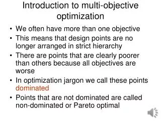
Introduction to multi-objective optimization • We often have more than one objective • This means that design points are no longer arranged in strict hierarchy • There are points that are clearly poorer than others because all objectives are worse • In optimization jargon we call these points dominated • Points that are not dominated are called non-dominated or Pareto optimal
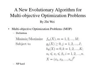
Definition of Pareto optimality • For a problem with m objective functions, a design variable vector x* is Pareto optimal if and only if there is no vector xin the feasible space with the characteristics
Problem domination • We have two objectives that are to be minimized. The following are the pairs of objectives at 10 design points. Mark the non-dominated ones. • (67,71) (48,72) (29,88) (-106, 294) (32,13), (-120,163), (103,-30) (-78,114) (-80,143) (75,-171)
Work choice example Minimize time and maximize fun so that you make at least $100. Will need between 33.3 to 100 items. Time can vary from 66.7 minutes to 300. Fun can vary between 33.3 and 300.
Example task 2 is dominated. Tasks 1,3,4 are Pareto optimal
Solution by enumeration • In the range of four variables calculate time and fun for all combination that produce exactly $100 • Pareto front is upper boundary and it is almost a straight line. • Matlab code given in note page.
Pay-fun Problem • Formulate the problem of maximizing fun and pay for five hours (300 minutes). • Obtain the Pareto front by enumeration and plot. • Write the equation for the Pareto front (fun as function of pay).
More efficient solution methods • Methods that try to avoid generating the Pareto front • Generate “utopia point” • Define optimum based on some measure of distance from utopia point • Generating entire Pareto front • Weighted sum of objectives with variable coefficients • Optimize one objective for a range of constraints on the others • Niching methods with population based algorithms
The utopia point is (66.7,300). One approach is to use it to form a compromise objective as shown above. It gives time=168 minutes, fun=160 (x3=76,x4=8)
Series of constraints The next slides provides a Matlab segment for solving this optimization problem using the function fmincon.
Matlab segment x0 = [10 10 10 10]; for fun_idx = 30:5:300 A = [-1 -2 -1 -3; -3 -2 -2 -1]; b = [-100;-fun_idx]; lb = zeros(4,1); options = optimset('Display','off'); [x,fval,exitflag,output,lambda] = fmincon('myfun',x0,A,b,[],[],lb,[],[],options); pareto_sol(fun_idx,:) = x; pareto_fun(fun_idx,1) = fval; pareto_fun(fun_idx,2) = 3*x(1) + 2*x(2) + 2*x(3) + x(4); End function f = myfun(x) f = 3*x(1) + 4*x(2) + 2*x(3) + 2*x(4);
Pareto-front Problem • Generate the Pareto front for the pay and fun maximization using a series of constraints, and also find a compromise point on it using the utopia point. • What is responsible for the slope discontinuity in the Pareto front on Slide 10?