Multi-objective Optimization of Earth Observing Satellite Missions
680 likes | 901 Vues
Multi-objective Optimization of Earth Observing Satellite Missions. By Panwadee Tangpattanakul Thesis supervisors Pierre Lopez Nicolas Jozefowiez 26 th September 2013. Agile Earth observing satellite (agile EOS). Mission

Multi-objective Optimization of Earth Observing Satellite Missions
E N D
Presentation Transcript
Multi-objective Optimization of Earth Observing Satellite Missions By PanwadeeTangpattanakul Thesis supervisors Pierre Lopez Nicolas Jozefowiez 26th September 2013
Agile Earth observing satellite (agile EOS) • Mission • Obtain photographs of the Earth surface to satisfy users requirements Satellitedirection Captured photograph Candidate photographs Earth surface
Work overview • Observation scheduling problem of agile EOS • & • Multi-objective optimization Biased random key genetic algorithm (BRKGA) Indicator-based multi-objective local search (IBMOLS) 3
Outline • Problem statement • Multi-objective optimization • Biased random key genetic algorithm • Indicator-based multi-objective local search • BRKGA vs. IBMOLS • Conclusions & perspectives
Properties of agile EOS • Ex. PLEIADES • CNES (French Center for Space Studies) • One fixed camera on-board • The whole satellite can move in 3 degrees of freedom 6
Literature of PLEIADES observation scheduling problem • Problem data’s description was proposed (Verfaillie et al., 2002) • Several methods were used to solve the problem, e.g. greedy algorithm, dynamic programming, constraint programming, local search (Lemaître et al., 2002) • ROADEF 2003 challenge • Simulated annealing (Kuipers, 2003) • Tabu search (Cordeau & Laporte, 2005) 7
Multi-user observation scheduling problem for agile EOS User 1 User 2 User n Ground station Requests Satellite capacity limitation Select Profit & Schedule Acquisitions
Multi-user observation scheduling problem for agile EOS • Literature • Bataille et al., 1999 • Optimize 2 objectives: fairness and efficiency • Use 3 strategies: • Give priority to fairness • Give priority to efficiency • Consider 2 objectives, but search for 1 solution • Gabrel & Vanderpooten, 2002 • Optimize 3 objectives: maximize the number of shots, maximize the total profit, and minimize the satellite use • Select a satisfactory efficient path in a graph without circuit
Multi-user observation scheduling problem for agile EOS • Literature • Bianchessi et al., 2007 • Multiple satellites, multiple orbits, and multiple users • 3 phases • Select users depending on priority • Select requests from the subset of users • Allocate the remaining capacities of the satellites between all users • A single objective: • Weighted sum of the normalized utilities of the users • Tabu search
Multi-user observation scheduling problem for agile EOS • The obtained sequence has to optimize 2 objectives: Sequence (SA1, SA2,…, SAn) • Maximize the total profit • Minimize the maximum profit difference between users • ensure fairness of resource sharing
Multi-user observation scheduling problem for agile EOS • Constraints • Time windows • No overlapping acquisitions Duration time Acquisition Possible starting time time Acquisition1 12 Acquisition2 time
Multi-user observation scheduling problem for agile EOS • Constraints • Sufficient transition times Earth surface 13
Multi-user observation scheduling problem for agile EOS • Constraints • Two acquisitions may be exclusive • Two acquisition may be linked Acqusition2E Acqusition1E time Acqusition1L Acqusition2L 14 time
Multi-user observation scheduling problem for agile EOS Request from P3 = 20 Acq3-1L P4= 10 User 2 Acq3-2L Acq4 P2-2= 5 P1= 4 Acq2-2E User 1 Acq1 Acq2-1E P2-1= 5 Time Max profit difference Solution 1: (Acq3-1L & Acq3-2L & Acq4) Total profit = 30, Max profit difference = 30 Solution 2: (Acq1 & Acq2-1E & Acq4) Total profit = 19, Max profit difference = 1 Solution 3: (Acq3-1L & Acq3-2L& Acq2-1E) Total profit = 25, Max profit difference = 15 Total profit
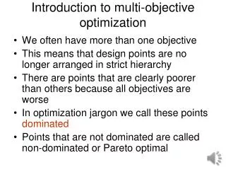
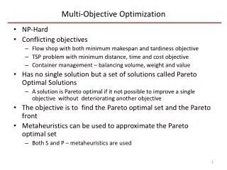
Multi-objective problem with: • n ≥2: number of objectives • F = (f1, f2,…,fn): vector of functions to optimize • Ω: set of feasible solutions • y = F(Ω): objective space
Pareto dominance & Hypervolume The considered problem needs to maximizef1 (x), minimizef2(x) A solution x dominates a solution yiff f1 (x) and f2(x) or f1 (x) and f2(x) f2(x) f2(x) Reference point E E D B C C A A f1 (x) f1(x)
Implementation • Conduct on realistic instances 4-user modified ROADEF 2003 challenge instances (Subset A) • The instance sizes are between 4 to 1,068 acquisitions • Implement via C++ language • 10 runs/instance are tested • Reference point of the hypervolume • The worst values of both objectives
Biased random key genetic algorithm Gonçalves et al. (2002) Random key (Bean, 1994) Chromosomes are represented as a vector of randomly generated real numbers in the interval [0,1]. Decision variable Encoding Chromosome Solution Decoding
Encoding Request from Acq3-1L User 2 Acq3-2L Acq4 Acq2-2E User 1 Acq1 Acq2-1E Time Random key chromosome
Biased random key genetic algorithm Gonçalves et al. (2002) Random key (Bean, 1994) Chromosomes are represented as a vector of randomly generated real numbers in the interval [0,1]. Decision variable Encoding Chromosome Solution Decoding
Decoding Multi-user observation scheduling problem Ordered list of acquisitions Sequence of selected acquisitions Random key chromosome Priority computation Assign the acquisition, which satisfies all constraints
Priority computation • Basic decoding (D1) • The priority is equal to its gene value Priorityj = genej • The priority to assign each acquisition in the sequence Acq2-1E,Acq3-2L, Acq1,Acq2-2E, Acq4,Acq3-1L Example Random key chromosome
Priority computation • Decoding of gene value and ideal priority combination (D2) • The priority is Priorityj = ideal priority * f(genej) • Concept of ideal priority • Theacquisition, which has the earliest possible starting time, should be selected firstly and be scheduled in the beginning of the solution sequence
Priority computation • The ideal priority values of Acq3-1L=Acq3-2L>Acq1>Acq2-1E>Acq2-2E > Acq4 Example Request from Acq3-1L User 2 Acq3-2L Acq4 Acq2-2E User 1 Acq1 Acq2-1E Time
Decoding Multi-user observation scheduling problem Ordered list of acquisitions Sequence of selected acquisitions Random key chromosome Priority computation Assign the acquisition, which satisfies all constraints
BRKGA generation POPULATION ELITE ELITE NON-ELITE CROSSOVER OFFSPRING X MUTANT Generation i Generation i+1
Adaptation to multi-objective • Q: How to select the elite set? A: Borrow selection methods from efficient MOEAs, e.g. NSGA-II, SMS-EMOA, IBEA • Q: Could chromosome be associated to several nondominated solutions? A: Use a multiple decoding
Elite set selections • Fast nondominated sorting and crowding distance assignment f2(x) Rank1 Rank2 Rank3 f1 (x) Ref: Deb et al. (2002)
Elite set selections • Fast nondominated sorting and crowding distance assignment Rank 1 Nondominated solutions f2(x) i+1 i i-1 f1 (x) solutions in Rank 1 Ref: Deb et al. (2002)
Elite set selections • S-metric selection evolutionary multiobjective optimization algorithm (SMS-EMOA) Rank 1 Nondominated solutions f2(x) solutions in Rank 1 f1 (x) Ref: Beume et al. (2007)
Elite set selections • Indicator-based evolutionary algorithm based on the hypervolumeconcept (IBEA) IHD(B,A)> 0 f2(x) f2(x) A A B B IHD(A,B) = -IHD(B,A)> 0 IHD(A,B)> 0 f1 (x) f1 (x) Binary tournament on all individuals in P Compute the fitness Ref: Zitzler et al. (2004)
Adaptation to multi-objective • Q: How to select the elite set? A: Borrow selection methods from efficient MOEAs, e.g. NSGA-II, SMS-EMOA, IBEA • Q: Could chromosome be associated to several nondominated solutions? A: Use a multiple decoding
Multiple Decoding • Hybrid decoding (HD) Chromosome Decoding of gene value and ideal priority combination (D2) Basic decoding (D1) Solution 1 Solution 2 ?
Hybrid decoding • Elite set management – Method 1 (M1) Population chromosome Preferredchromosomes Elite set D1 D2 solution 1 solution 2 Dominance relation Dominant solution
Hybrid decoding • Elite set management – Method 1 (M1) Population chromosome Preferredchromosomes Elite set D1 D2 solution 1 solution 2 Select randomly Selected solution
Hybrid decoding • Elite set management – Method 2 (M2) Preferredchromosomes Elite set Population solution 1 D1 chromosome D2 solution 2
Hybrid decoding • Elite set management – Method 3 (M3) Preferred chr. Elite set Population D1 solution 1 chromosome Preferred chr. D2 solution 2
Implementation • In each iteration, • Nondominated solutions are stored in an archive set A • If at least one solution from P can dominate some solutions in the archive set A • Update the archive set A
Implementation • Stopping criteria • Number of iterations since the last archive improvement • Value = 50 • Computation time limitation • Depending on the instances size
Comparison of two decodings (D1, D2) and three elite set selections (S1, S2, and S3) S1, S2, and S3 • For all instances • All methods obtain similar results • Each method has the advantage in different instances
Comparison of two decodings (D1, D2) and three elite set selections (S1, S2, and S3) D1, D2 • Medium-size instances • D2 obtains better results • Median value • Std. deviation • Computation time • Large-size instances • D1 obtains better median • value • D2 can reduce the range
Hybrid decoding – Comparison of elite set management Since M1 spends less computation time for all elite set selection methods, its results will be used to compare with the results from the two single decoding
BRKGA – Comparison of two single decoding and hybrid decoding • HD obtains results close to the best one, when comparing the two single decoding • HD can preserve the advantages of each single decoding • D1 vs. HD, HD can reduce the range • D2 vs. HD, HD can avoid to entrap in local optima
Indicator-based multi-objective local search (Basseurand Burke, 2007) Basic Local search & Binary indicator from IBEA Each iteration Update the approximate Pareto front Initial population generation Fitness computation Local search step
Strategies • Initial population generation First iteration • Random generation • Using data of problem instances Other iterations • Random generation • Perturbation • Neighborhood structure and dynamic stopping value • Insert, remove, and replace & Stop value = 10 • Insert, remove & Stop value = 10 • Insert, remove & Stop value = 50
Strategies • Feasibility checking • Method 1 • Method 2 • Stopping criterion • Dynamic stopping • Fixed computation time • Fixed number of visited neighbors