Likelihood, Bayesian & Decision Theory Overview
500 likes | 548 Vues
Explore the application and importance of Maximum Likelihood, Bayesian, and Decision Theory in scientific research. Learn about estimating unknown parameters, MLE, Fisher information, Cramér-Rao bound, and likelihood ratio tests.

Likelihood, Bayesian & Decision Theory Overview
E N D
Presentation Transcript
Chapter 15: Likelihood, Bayesian, and Decision Theory AMS 572 Group Members Yen-hsiu Chen, Valencia Joseph, Lola Ojo, Andrea Roberson, Dave Roelfs, Saskya Sauer, Olivia Shy, Ping Tung
Introduction "To call in the statistician after the experiment is done may be no more than asking him to perform a post-mortem examination: he may be able to say what the experiment died of." - R.A. Fisher • Maximum Likelihood, Bayesian, and Decision Theory are applied and have proven its selves useful and necessary in sciences, such as physics, as well as research in general. • They provide a practical way to begin and carry out an analysis or experiment.
15.1.1 Likelihood Function • Objective : Estimating the unknown parameters θof a population distribution based on a random sample χ1,…,χn from that distribution • Previous chapters : Intuitive Estimates => Sample Means for Population Mean • To improve estimation, R. A. Fisher (1890~1962) proposed MLE in 1912~1922.
Ronald Aylmer Fisher (1890~1962) • The greatest of Darwin's successors • Known for : • 1912 : Maximum likelihood • 1922 : F-test • 1925 : Analysis of variance (Statistical Method for Research Workers ) • Notable Prizes : • Royal Medal (1938) • Copley Medal (1955) Source: http://www-history.mcs.st-andrews.ac.uk/history/PictDisplay/Fisher.html
Joint p.d.f. vs. Likelihood Function • Identical quantities • Different interpretation • Joint p.d.f. of X1 ,…, Xn : • A function of χ1,…,χn for given θ • Probability interpretation • Likelihood Function of θ : • A function of θfor givenχ1,…,χn • No probability interpretation
Example : Normal Distribution • Suppose χ1,…,χn is a random sample from a normal distribution with p.d.f.: parameter ( ), Likelihood Function:
15.1.2 Calculation of Maximum Likelihood Estimators (MLE) • MLE of an unknown parameter θ: The value which maximizes the likelihood function • Example of MLE: • 2 independent Bernoulli trials with success probability θ • θis known : 1/4 and 1/3 =>parameter space Θ= {1/4, 1/3} • Using Binomial distribution, the probabilities of observing χ= 0, 1, 2 successes can be calculated
Example of MLE • Probability of ObservingχSuccesses • When χ=0, the MLE of • When χ=1 or 2, the MLE of • The MLE is chosen to maximize for observed χ
15.1.3 Properties of MLE’s • Objective optimality properties in large sample • Fisher information (continuous case) • Alternatives of Fisher information (1) (2)
MLE (Continued) • Define the Fisher information for an i.i.d. sample
MLE (Continued) • Generalization of the Fisher information for • k-dimensional vector parameter
MLE (Continued) • Cramér-Rao Lower Bound • A random sample X1, X2, …, Xn from p.d.f f(x|θ). • Let be any estimator of θ with where B(θ) is the bias of If B(θ) is differentiable in θ and if certain regularity conditions holds, then • (Cramér-Rao inequality) • The ratio of the lower bound to the variance of any estimator of θ is called the efficiency of the estimator. • An estimator has efficiency = 1 is called the efficient estimator.
15.1.4 Large Sample Inference Based on the MLE’s Large sample inference on unknown parameter θ • estimate • 100(1-α)% CI for θ
15.1.4 Delta Method for Approximating the Variance of an Estimator • Delta method estimate a nonlinear function h(θ) suppose that and is a known function of θ. using
15.2 Likelihood Ratio Tests The last section presented an inference for pointwise estimation based on likelihood theory. In this section, we present a corresponding inference for testing hypotheses. Let be a probability density function where is a real valued parameter taking values in an interval that could be the whole real line. We call the parameter space. An alternative hypothesis will restrict the parameter to some subset of the parameter space . The null hypothesis is then the complement of with respect to .
Consider the two-sided hypothesis versus , where is a specified value. We will test versus on the basis of the random sample from . If the null hypothesis holds, we would expect the likelihood to be relatively large, when evaluated at the prevailing value . Consider the ratio of two likelihood functions, namely Note that , but if is true should be close to 1; while if is true, should be smaller. For a specified significance level , we have the decision rule, reject in favor of if , where c is such that This test is called the likelihood ratio test.
Example 1 Let be a random sample of size n from a normal distribution with known variance. Obtain the likelihood ratio for testing versus . So is a maximum since . < 0 . Thus is the MLE of .
Example 1 (continued) . is equivalent to thus
Example 2 Let be a random sample from a Poisson distribution with mean >0. a. Show that the likelihood ratio test of versus is based upon the statistic . Obtain the null distribution of Y. So is a maximum since thus is the mle of
Example 2 (continued) The likelihood ratio test statistic is: = = = , . Under And it’s a function of Y =
Example 2 (continued) • For = 2 and n = 5, find the significance level of the test that rejects if or . The null distribution of Y is Poisson(10).
Composite Null Hypothesis The likelihood ratio approach has to be modified slightly when the null hypothesis is composite. When testing the null hypothesis concerning a normal mean when is unknown, the parameter space is a subset of The null hypothesis is composite and Since the null hypothesis is composite, it isn’t certain which value of the parameter(s) prevails even under . So we take the maximum of the likelihood over The generalized likelihood ratio test statistic is defined as
Example 3 be a random sample of size n from a normal distribution with unknown mean and variance. Obtain the likelihood ratio test statistic for testing Let versus In Example 1, we found the unrestricted mle: Now = , Since we only need to find the value of maximizing
Example 3 (continued) So is a maximum since is the MLE of Thus Thus is the MLE of We can also write .
Example 3 (continued) Rejection region: , such that so where define and implies or So where
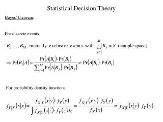
15.3 : Bayesian Inference Bayesian inference refers to a statistical inference where new facts are presented and used draw updated conclusions on a prior belief. The term ‘Bayesian’ stems from the well known Bayes Theorem which was first derived by Reverend Thomas Bayes. Thomas Bayes (c. 1702 – April 17, 1761) Source: www.wikipedia.com Thomas Bayes(pictured above) was a Presbyterian minister and a mathematician born in London who developed a special case of Bayes’ theorem which was published and studied after his death. f (A|B) = f (A ∩ B) / f (B) = f (B | A) f (A) /f(B) since, f (A ∩ B)= f (B ∩ A) = f (B | A) f (A) Bayes’ Theorem (review): (15.1)
Some Key Terms in Bayesian Inference… …in plain English • prior distribution – probability tendency of an uncertain quantity, θ, that expresses previous knowledge of θ from, for example, a past experience, with the absence of some proof • posterior distribution – this distribution takes proof into account and is then the conditional probability of θ. The posterior probability is computed from the prior and the likelihood function using Bayes’ theorem. • posterior mean – the mean of the posterior distribution • posterior variance – the variance of the posterior distribution • conjugate priors - a family of prior probability distributions in which the key property is that the posterior probability distribution also belongs to the family of the prior probability distribution
15.3.1 Bayesian Estimation So far we’ve learned that the Bayesian approach treats θ as a random variable and then data is used to update the prior distribution to obtain the posterior distribution of θ. Now lets move on to how we can estimate parameters using this approach. (Using text notation) Let θ be an unknown parameter based on a random sample, x1, x2, …, xnfrom a distribution with pdf/pmf f (x | θ). Let π (θ) be the prior distribution of θ. Let π *(θ | x1, x2, …, xn) be the posterior distribution. **Note that π *(θ | x1, x2, …, xn) is the condition distribution of θ given the observed data, x1, x2, …, xn. If we apply Bayes Theorem (Eq. 15.1), ourposterior distributionbecomes: f(x1, x2, …, xn | θ)π(θ) f(x1, x2, …, xn | θ)π(θ) = (15.2) f *(θ | x1, x2, …, xn) f (x1, x2, …, xn | θ)π(θ) dθ *Note that f *(θ | x1, x2, …, xn) is the marginal PDF of X1, X2, …,Xn
Bayesian Estimation (continued) As seen in equation 15.2, the posterior distribution represents what is known about θ after observing the data X = x1, x2, …, xn . From earlier chapters, we know that the likelihood of a variable θ isf (X | θ) . So, to get a better idea of the posterior distribution, we note that: posterior distribution likelihood x prior distribution i.e. π *(θ | X)f (X | θ)xπ(θ) For a detailed practical example of deriving the posterior mean and using Bayesian estimation, visit: http://www.stat.berkeley.edu/users/rice/Stat135/Bayes.pdf ☺
Example 15.26 Let x be the number of successes from n i.i.d. Bernoulli trials with unknown success probability p=θ. Show that the beta distribution is a conjugate prior on θ. ★ ★ ★ Goal
Example 15.26 (continued) X has a binominal distribution of n and p= θ x=1,2…,n Prior distribution of θis the beta distribution 0≤ θ ≥1
Example 15.26 (continued) It is a beta distribution with parameters (x+a) and (n-x+b)!!
Notes: The parameters a and b of the prior distribution may be interpreted as prior successes and prior failures, with m=a+b being the total number of prior observations. After actually observing x successes and n-x failures in n i.i.d Bernoulli trials, these parameters are updated to a+x and b+n-x, respectively. The prior and posterior means are, respectively, and
15.3.2 Bayesian Testing Assumption: , we reject in favor of . If Where k >0 is a suitably chosen critical constant.
15.4 Decision Theory Abraham Wald (1902-1950) was the founder of Statistical decision theory. His goal was to provide a unified theoretical framework for diverse problems. i.e. point estimation, confidence interval estimation and hypothesis testing. Source: http://www-history.mcs.st-andrews.ac.uk/history/PictDisplay/Wald.html
Statistical Decision Problem • The goal: is to choose a decision d from a set of possible decisions D, based on a sample outcome (data) x • Decision space is D • Sample space: the set of all sample outcomes denoted by x • Decision Rule:δ is a function δ(x) which assigns to every sample outcome x є X, a decision dєD.
Continued… • Denote by X the R.V. corresponding to x and the probability distribution of X by f (x|θ). • The above distribution depends on an unknown parameter θbelonging to a parameter space Θ • Suppose one chooses a decision d when the true parameter is θ, a loss of L (d, θ) is incurred also known as the loss function. • The decision rule is assessed by evaluating its expectedloss called the risk function: R(δ, θ) = E[L(δ(X),θ)] = ∫xL(δ(X),θ) f (x|θ)dx.
Example • Calculate and compare the risk functions for the squared error loss of two estimators of success probability p from n i.i.d. Bernoulli trials. The first is the usual sample proportion of successes and the second is the bayes estimator from Example 15.26: ṗ1 = X/n and ṗ2 = a + X/ m + n
Von Neumann (1928): Minimax Source:http://jeff560.tripod.com/
How Minimax Works • Focuses on risk avoidance • Can be applied to both zero-sum and non-zero-sum games • Can be applied to multi-stage games • Can be applied to multi-person games
Classic Example: The Prisoner’s Dilemma • Each player evaluates his/her alternatives, attempting to minimize his/her own risk • From a common sense standpoint, a sub-optimal equilibrium results
Classic example: With Probabilities • When disregarding the probabilities when playing the game, (D,B) is the equilibrium point under minimax • With probabilities (p=q=r=1/4), player one will choose B. This is…
…how Bayes works • View {(pi,qi,ri)} as θi where i=1 in the previous example • Letting i=[1,n] we get a much better idea of what Bayes meant by “states of nature” and how probabilities of each state enter into one’s strategy
Conclusion We covered three theoretical approaches in our presentation • Likelihood • provides statistical justification for many of the methods used in statistics • MLE - method used to make inferences about parameters of the underlying probability distribution of a given data set • Bayesian and Decision Theory • paradigms used in statistics • Bayesian Theory • probabilities are associated with individual event or statements rather than with sequences of events • Decision Theory • Describe and rationalize the process of decision making, that is, making a choice of among several possible alternatives Source: http://www.answers.com/maximum%20likelihood,http://www.answers.com/bayesian%20theory, http://www.answers.com/decision%20theory
The End Any questions for the group?
