Data Intensive Cyberinfrastructure
The rapid evolution of technology is reshaping the landscape of data-intensive cyberinfrastructure. This presentation highlights the growing significance of CPUs and cloud environments compared to traditional grids. By comparing bioinformatics and information retrieval, we outline the distinct architectural approaches to data analysis/mining versus large-scale simulations. A critical examination of MapReduce and MPI is conducted, suggesting possible integrated runtime approaches. Performance assessments between commercial clouds and traditional clusters, alongside the innovative capabilities of FutureGrid, reveal key trends in cloud technology and data science applications.


Data Intensive Cyberinfrastructure
E N D
Presentation Transcript
Data Intensive Cyberinfrastructure Geoffrey Fox gcf@indiana.edu http://www.infomall.orghttp://www.futuregrid.org Director, Digital Science Center, Pervasive Technology Institute Associate Dean for Research and Graduate Studies, School of Informatics and Computing Indiana University Bloomington University of Tennessee, Knoxsville August 26 2010
Data Intensive Cyberinfrastructure • AbstractThe technology landscape is changing rapidly with CPU and clouds growing in importance compared to Grids. On the application side, the data deluge is bringing new computational challenges and opportunities. We use bioinformatics and information retrieval to contrast the architecture differences between data analysis/mining and large scale simulation. We critique MapReduce and MPI and suggest that runtimes interpolating between these paradigms are appropriate. Performance results compare commercial clouds and traditional clusters and we highlight FutureGrid as a platform to explore these emerging ideas..
Layout of the Talk • Important Trends • Cloud Technologies • Data Intensive Science Applications • Use of Clouds • Algorithms • FutureGrid
Important Trends • Data Deluge in all fields of science • Multicoreimplies parallel computing important again • Performance from extra cores – not extra clock speed • GPU enhanced systems can give big power boost • Clouds – new commercially supported data center model replacing compute grids (and your general purpose computer center) • Light weight clients: Sensors, Smartphones and tablets accessing and supported by backend services in cloud • Commercial efforts moving much faster than academia in both innovation and deployment
Gartner 2009 Hype Curve Clouds, Web2.0 Service Oriented Architectures
Data Centers Clouds & economies of scale Range in size from “edge” facilities to megascale. Economies of scale Approximate costs for a small size center (1K servers) and a larger, 50K server center. Each data center is 11.5 times the size of a football field 2 Google warehouses of computers on the banks of the Columbia River, in The Dalles, Oregon Such centers use 20MW-200MW (Future) each with 150 watts per CPU Save money from large size, positioning with cheap power and access with Internet
Data Centers, Clouds & economies of scale II • Builds giant data centers with 100,000’s of computers; ~ 200-1000 to a shipping container with Internet access • “Microsoft will cram between 150 and 220 shipping containers filled with data center gear into a new 500,000 square foot Chicago facility. This move marks the most significant, public use of the shipping container systems popularized by the likes of Sun Microsystems and Rackable Systems to date.”
Amazon offers a lot! The Cluster Compute Instances use hardware-assisted (HVM) virtualization instead of the paravirtualization used by the other instance types and requires booting from EBS, so you will need to create a new AMI in order to use them. We suggest that you use our Centos-based AMI as a base for your own AMIs for optimal performance. See the EC2 User Guide or the EC2 Developer Guide for more information. The only way to know if this is a genuine HPC setup is to benchmark it, and we've just finished doing so. We ran the gold-standard High Performance Linpack benchmark on 880 Cluster Compute instances (7040 cores) and measured the overall performance at 41.82 TeraFLOPS using Intel's MPI (Message Passing Interface) and MKL (Math Kernel Library) libraries, along with their compiler suite. This result places us at position 146 on the Top500 list of supercomputers. The input file for the benchmark is here and the output file is here.
Philosophy of Clouds and Grids • Clouds are (by definition) commercially supported approach to large scale computing • So we should expect Clouds to replace Compute Grids • Current Grid technology involves “non-commercial” software solutions which are hard to evolve/sustain • Maybe Clouds ~4% IT expenditure 2008 growing to 14% in 2012 (IDC Estimate) • Public Clouds are broadly accessible resources like Amazon and Microsoft Azure – powerful but not easy to customize and perhaps data trust/privacy issues • Private Clouds run similar software and mechanisms but on “your own computers” (not clear if still elastic) • Platform features such as Queues, Tables, Databases limited • Services still are correct architecture with either REST (Web 2.0) or Web Services • Clusters still critical concept
X as a Service • SaaS: Software as a Service imply software capabilities (programs) have a service (messaging) interface • Applying systematically reduces system complexity to being linear in number of components • Access via messaging rather than by installing in /usr/bin • IaaS: Infrastructure as a Service or HaaS: Hardware as a Service – get your computer time with a credit card and with a Web interface • PaaS: Platform as a Service is IaaS plus core software capabilities on which you build SaaS • Cyberinfrastructureis“Research as a Service” • SensaaS is Sensors (Instruments) as a Service (cf. Data as a Service) Other Services Clients
Grids and Clouds + and - • Grids are useful for managing distributed systems • Pioneered service model for Science • Developed importance of Workflow • Performance issues – communication latency – intrinsic to distributed systems • Clouds can execute any job class that was good for Grids plus • More attractive due to platform plus elasticity • Currently have performance limitations due to poor affinity (locality) for compute-compute (MPI) and Compute-data • These limitations are not “inevitable” and should gradually improve
Cloud Computing: Infrastructure and Runtimes • Cloud infrastructure: outsourcing of servers, computing, data, file space, utility computing, etc. • Handled through Web services that control virtual machine lifecycles. • Cloud runtimes or Platform:tools (for using clouds) to do data-parallel (and other) computations. • Apache Hadoop, Google MapReduce, Microsoft Dryad, Bigtable, Chubby and others • MapReduce designed for information retrieval but is excellent for a wide range of science data analysis applications • Can also do much traditional parallel computing for data-mining if extended to support iterative operations • MapReduce not usually on Virtual Machines
Reduce(Key, List<Value>) Map(Key, Value) MapReduce • Implementations (Hadoop – Java; Dryad – Windows) support: • Splitting of data • Passing the output of map functions to reduce functions • Sorting the inputs to the reduce function based on the intermediate keys • Quality of service Data Partitions A hash function maps the results of the map tasks to reduce tasks Reduce Outputs
MapReduce “File/Data Repository” Parallelism Map = (data parallel) computation reading and writing data Reduce = Collective/Consolidation phase e.g. forming multiple global sums as in histogram Instruments Communication Iterative MapReduce Map MapMapMap Reduce ReduceReduce Portals/Users Reduce Map1 Map2 Map3 Disks
High Energy Physics Data Analysis An application analyzing data from Large Hadron Collider(1TB but 100 Petabytes eventually) Input to a map task: <key, value> key = Some Id value = HEP file Name Output of a map task: <key, value> key = random # (0<= num<= max reduce tasks) value = Histogram as binary data Input to a reduce task: <key, List<value>> key = random # (0<= num<= max reduce tasks) value = List of histogram as binary data Output from a reduce task: value value = Histogram file Combine outputs from reduce tasks to form the final histogram
Reduce Phase of Particle Physics “Find the Higgs” using Dryad • Combine Histograms produced by separate Root “Maps” (of event data to partial histograms) into a single Histogram delivered to Client Higgs in Monte Carlo
Broad Architecture Components • Traditional Supercomputers (TeraGrid and DEISA) for large scale parallel computing – mainly simulations • Likely to offer major GPU enhanced systems • Traditional Grids for handling distributed data – especially instruments and sensors • Clouds for “high throughput computing” including much data analysis and emerging areas such as Life Sciences using loosely coupled parallel computations • May offer small clusters for MPI style jobs • Certainly offer MapReduce • Integrating these needs new work on distributed file systems and high quality data transfer service • Link Lustre WAN, Amazon/Google/Hadoop/Dryad File System • Offer Bigtable (distributed scalable Excel)
Application Classes Old classification of Parallel software/hardware in terms of 5 (becoming 6) “Application architecture” Structures)
Applications & Different Interconnection Patterns Input map iterations Input Input map map Output Pij reduce reduce Domain of MapReduce and Iterative Extensions MPI
Fault Tolerance and MapReduce • MPI does “maps” followed by “communication” including “reduce” but does this iteratively • There must (for most communication patterns of interest) be a strict synchronization at end of each communication phase • Thus if a process fails then everything grinds to a halt • In MapReduce, all Map processes and all reduce processes are independent and stateless and read and write to disks • As 1 or 2 (reduce+map) iterations, no difficult synchronization issues • Thus failures can easily be recovered by rerunning process without other jobs hanging around waiting • Re-examine MPI fault tolerance in light of MapReduce • Twister will interpolate between MPI and MapReduce
DNA Sequencing Pipeline MapReduce Illumina/Solexa Roche/454 Life Sciences Applied Biosystems/SOLiD Pairwise clustering Blocking MDS MPI Modern Commercial Gene Sequencers Visualization Plotviz Sequence alignment Dissimilarity Matrix N(N-1)/2 values block Pairings FASTA FileN Sequences Read Alignment Internet • This chart illustrate our research of a pipeline mode to provide services on demand (Software as a Service SaaS) • User submit their jobs to the pipeline. The components are services and so is the whole pipeline.
Alu and Metagenomics Workflow “All pairs” problem Data is a collection of N sequences. Need to calculate N2dissimilarities (distances) between sequnces (all pairs). • These cannot be thought of as vectors because there are missing characters • “Multiple Sequence Alignment” (creating vectors of characters) doesn’t seem to work if N larger than O(100), where 100’s of characters long. Step 1: Can calculate N2 dissimilarities (distances) between sequences Step 2: Find families by clustering (using much better methods than Kmeans). As no vectors, use vector free O(N2) methods Step 3: Map to 3D for visualization using Multidimensional Scaling (MDS) – also O(N2) Results: N = 50,000 runs in 10 hours (the complete pipeline above) on 768 cores Discussions: • Need to address millions of sequences ….. • Currently using a mix of MapReduce and MPI • Twister will do all steps as MDS, Clustering just need MPI Broadcast/Reduce
Alu Families This visualizes results of Alu repeats from Chimpanzee and Human Genomes. Young families (green, yellow) are seen as tight clusters. This is projection of MDS dimension reduction to 3D of 35399 repeats – each with about 400 base pairs
Metagenomics This visualizes results of dimension reduction to 3D of 30000 gene sequences from an environmental sample. The many different genes are classified by clustering algorithm and visualized by MDS dimension reduction
All-Pairs Using DryadLINQ 125 million distances 4 hours & 46 minutes • Calculate pairwise distances for a collection of genes (used for clustering, MDS) • Fine grained tasks in MPI • Coarse grained tasks in DryadLINQ • Performed on 768 cores (Tempest Cluster) Calculate Pairwise Distances (Smith Waterman Gotoh) Moretti, C., Bui, H., Hollingsworth, K., Rich, B., Flynn, P., & Thain, D. (2009). All-Pairs: An Abstraction for Data Intensive Computing on Campus Grids. IEEE Transactions on Parallel and Distributed Systems, 21, 21-36.
Hadoop/Dryad ComparisonInhomogeneous Data I Inhomogeneity of data does not have a significant effect when the sequence lengths are randomly distributed Dryad with Windows HPCS compared to Hadoop with Linux RHEL on Idataplex (32 nodes)
Hadoop/Dryad ComparisonInhomogeneous Data II This shows the natural load balancing of Hadoop MR dynamic task assignment using a global pipe line in contrast to the DryadLinq static assignment Dryad with Windows HPCS compared to Hadoop with Linux RHEL on Idataplex (32 nodes)
Hadoop VM Performance Degradation Perf. Degradation = (Tvm – Tbaremetal)/Tbaremetal 15.3% Degradation at largest data set size
Twister(MapReduce++) Pub/Sub Broker Network Map Worker M Static data Configure() • Streaming based communication • Intermediate results are directly transferred from the map tasks to the reduce tasks – eliminates local files • Cacheablemap/reduce tasks • Static data remains in memory • Combine phase to combine reductions • User Program is the composer of MapReduce computations • Extendsthe MapReduce model to iterativecomputations Worker Nodes Reduce Worker R D D MR Driver User Program Iterate MRDeamon D M M M M Data Read/Write R R R R User Program δ flow Communication Map(Key, Value) File System Data Split Reduce (Key, List<Value>) Close() Combine (Key, List<Value>) Different synchronization and intercommunication mechanisms used by the parallel runtimes
Iterative Computations K-means Matrix Multiplication Smith Waterman Performance of K-Means Performance Matrix Multiplication
Performance of Pagerank using ClueWeb Data (Time for 20 iterations)using 32 nodes (256 CPU cores) of Crevasse
Matrix Multiplication 32 nodes 8 nodes
TwisterMPIReduce • Runtime package supporting subset of MPI mapped to Twister • Set-up, Barrier, Broadcast, Reduce PairwiseClusteringMPI • Multi Dimensional Scaling MPI • Generative Topographic Mapping MPI • Other … TwisterMPIReduce Azure Twister (C# C++) Java Twister Microsoft Azure • FutureGrid • Amazon EC2 • Local Cluster
2916 iterations (384 CPUcores) 968 iterations (384 CPUcores) 343 iterations (768 CPU cores)
Sequence Assembly in the Clouds Cap3 parallel efficiency Cap3– Per core per file (458 reads in each file) time to process sequences
Applications using Dryad & DryadLINQ Input files (FASTA) CAP3 - Expressed Sequence Tag assembly to re-construct full-length mRNA • Perform using DryadLINQ and Apache Hadoop implementations • Single “Select” operation in DryadLINQ • “Map only” operation in Hadoop CAP3 CAP3 CAP3 DryadLINQ Output files X. Huang, A. Madan, “CAP3: A DNA Sequence Assembly Program,” Genome Research, vol. 9, no. 9, pp. 868-877, 1999.
Early Results with AzureMapreduce Compare Hadoop - 4.44 ms Hadoop VM - 5.59 ms DryadLINQ - 5.45 ms Windows MPI - 5.55 ms
Currently we can’t make Amazon Elastic MapReduce run well • Hadoop runs well on Xen FutureGrid Virtual Machines
Some Issues with AzureTwister and AzureMapReduce • Transporting data to Azure: Blobs (HTTP), Drives (GridFTP etc.), Fedex disks • Intermediate data Transfer: Blobs (current choice) versus Drives (should be faster but don’t seem to be) • Azure Table v Azure SQL: Handle all metadata • Messaging Queues: Use real publish-subscribe system in place of Azure Queues • Azure Affinity Groups: Could allow better data-compute and compute-compute affinity
Parallel Data Analysis Algorithms on Multicore Developing a suite of parallel data-analysis capabilities • Clustering with deterministic annealing (DA) • Dimension Reduction for visualization and analysis (MDS, GTM) • Matrix algebraas needed • Matrix Multiplication • Equation Solving • Eigenvector/value Calculation
Deterministic Annealing Clustering (DAC) • F is Free Energy • EM is well known expectation maximization method • p(x) with p(x) =1 • T is annealing temperature varied down from with final value of 1 • Determine cluster centerY(k) by EM method • K (number of clusters) starts at 1 and is incremented by algorithm N data points E(x) in D dimensions space and minimize F by EM General Deterministic Annealing Formula
Deterministic Annealing I • Gibbs Distribution at Temperature TP() = exp( - H()/T) / d exp( - H()/T) • Or P() = exp( - H()/T + F/T ) • Minimize Free EnergyF= < H- T S(P) > = d {P()H+ T P() lnP()} • Where are (a subset of) parameters to be minimized • Simulated annealing corresponds to doing these integrals by Monte Carlo • Deterministic annealing corresponds to doing integrals analytically and is naturally much faster • In each case temperature is lowered slowly – say by a factor 0.99 at each iteration
DeterministicAnnealing • Minimum evolving as temperature decreases • Movement at fixed temperature going to local minima if not initialized “correctly F({y}, T) Solve Linear Equations for each temperature Nonlinearity effects mitigated by initializing with solution at previous higher temperature Configuration {y}
Deterministic Annealing II • For some cases such as vector clustering and Gaussian Mixture Models one can do integrals by hand but usually will be impossible • So introduce Hamiltonian H0(, ) which by choice of can be made similar to H() and which has tractable integrals • P0() = exp( - H0()/T + F0/T ) approximate Gibbs • FR (P0) = < HR - T S0(P0) >|0 = < HR – H0> |0 + F0(P0) • Where <…>|0denotes d Po() • Easy to show that real Free Energy FA (PA) ≤ FR (P0) • In many problems, decreasing temperature is classic multiscale – finer resolution (T is “just” distance scale) • Related to variational inference
Deterministic Annealing Clustering of Indiana Census Data Decrease temperature (distance scale) to discover more clusters Distance ScaleTemperature0.5 Redis coarse resolution with 10 clusters Blue is finer resolution with 30 clusters Clusters find cities in Indiana Distance Scale is Temperature
Implementation of DA I • Expectation step E is find minimizing FR (P0) and • Follow with M step setting = <> |0 = dPo() and if one does not anneal over all parameters and one follows with a traditional minimization of remaining parameters • In clustering, one then looks at second derivativematrixof FR (P0) wrtand as temperature is lowered this develops negative eigenvaluecorresponding to instability • This is a phase transition and one splits cluster into two and continues EM iteration • One starts with just one cluster