Two-Factor Full Factorial Design with Replications Overview
220 likes | 313 Vues
Learn about computation of effects, estimating experimental errors, ANOVA tables, confidence intervals, and more in this comprehensive guide on two-factor designs with replications.

Two-Factor Full Factorial Design with Replications Overview
E N D
Presentation Transcript
Two Factor Full Factorial Design with Replications Raj Jain Washington University in Saint LouisSaint Louis, MO 63130Jain@cse.wustl.edu These slides are available on-line at: http://www.cse.wustl.edu/~jain/cse567-08/
Overview • Model • Computation of Effects • Estimating Experimental Errors • Allocation of Variation • ANOVA Table and F-Test • Confidence Intervals For Effects
Model • Replications allow separating out the interactions from experimental errors. • Model: With r replications • Here,
Model (Cont) • The effects are computed so that their sum is zero: • The interactions are computed so that their row as well as column sums are zero: • The errors in each experiment add up to zero:
Computation of Effects • Averaging the observations in each cell: • Similarly, Use cell means to compute row and column effects.
Example 22.1: Computation of Effects • An average workload on an average processor requires a code size of 103.94 (8710 instructions). • Processor W requires 100.23 (=1.69) less code than avg processor. • Processor X requires 100.02 (=1.05) less than an average processor and so on. • The ratio of code sizes of an average workload on processor W and X is 100.21 (= 1.62).
Example 22.1: Interactions • Check: The row as well column sums of interactions are zero. • Interpretation: Workload I on processor W requires 0.02 less log code size than an average workload on processor W or equivalently 0.02 less log code size than I on an average processor.
Computation of Errors • Estimated Response: • Error in the kth replication: • Example 22.2: Cell mean for (1,1) = 3.8427 Errors in the observations in this cell are: 3.8455-3.8427 = 0.0028 3.8191-3.8427 = -0.0236, and 3.8634-3.8427 = 0.0208 Check: Sum of the three errors is zero.
Allocation of Variation • Interactions explain less than 5% of variation Þ may be ignored.
Analysis of Variance • Degrees of freedoms:
Example 22.4: Code Size Study • All three effects are statistically significant at a significance level of 0.10.
Confidence Intervals For Effects • Use t values at ab(r-1) degrees of freedom for confidence intervals
Example 22.5: Code Size Study • From ANOVA table: se=0.03. The standard deviation of processor effects: • The error degrees of freedom: ab(r-1) = 40 use Normal tables For 90% confidence, z0.95 = 1.645 90% confidence interval for the effect of processor W is: a1¨ t sa1 = -0.2304 ¨ 1.645 £ 0.0060 = -0.2304 ¨ 0.00987 = (-0.2406, -0.2203) The effect is significant.
Example 22.5: Conf. Intervals (Cont) • The intervals are very narrow.
Example 22.5: Visual Tests • No visible trend. • Approximately linear ) normality is valid.
Summary • Replications allow interactions to be estimated • SSE has ab(r-1) degrees of freedom • Need to conduct F-tests for MSA/MSE, MSB/MSE, MSAB/MSE
Exercise 22.1 Measured CPU times for three processors A1, A2, and A3, on five workloads B1, B2, through B5 are shown in the table. Three replications of each experiment are shown. Analyze the data and answer the following: • Are the processors different from each other at 90% level of confidence? • What percent of variation is explained by the processor-workload interaction? • Which effects in the model are not significant at 90% confidence.
Homework 22 • Submit answer to Exercise 22.1. Show all numerical values.