Two-level Factorial Designs
Two-level Factorial Designs. Bacteria Example: Response: Bill length Factors: B: Bacteria (Myco, Control) T: Room Temp (Warm, Cold) I: Inoculation (Eggs, Chicks) . Two-level Factorial Designs. +. 41.71. 40.78. W. 40.37. 40.21. Temp. 40.23. 38.95. C. Bacteria. C. 39.77. 39.19.


Two-level Factorial Designs
E N D
Presentation Transcript
Two-level Factorial Designs • Bacteria Example: • Response: Bill length • Factors: • B: Bacteria (Myco, Control) • T: Room Temp (Warm, Cold) • I: Inoculation (Eggs, Chicks) Yandell, B. (2002) Practical Data Analysis for Designed Experiments, Chapman & Hall, London
+ 41.71 40.78 W 40.37 40.21 Temp 40.23 38.95 C Bacteria C 39.77 39.19 E Inoculation C M Cube Plot
Estimated Effects • For a k-factor design with n replicates, the cell means are estimated as • We can write any effect as a contrast; interaction contrasts are obtained by element-wise multiplication of main effect contrast coefficients.
Estimated Effects • The resulting contrasts are mutually orthogonal. • The contrasts (up to a scaling constant) can be summarized as a table of ±1’s.
Estimated Effects • If we code contrast coefficients as ±1, the estimated effects are: • These effects are twice the size of our usual ANOVA effects.
Estimated Effects • The sum of squares for the estimated effect can be computed using the sum of squares formula we learned for contrasts
Estimated Effects • Bacteria Example B effect=(39.19+38.95+40.21+40.78-39.77-40.23-40.37-41.71)/4 =-.7375 SSB=(-.7375)2x2=1.088 • The entire ANOVA table for this example can be constructed in this way
Testing Effects • With replication (n>1) • Without replication (k large) • Claim higher-order interactions are negligible and pool them • For k=6, if 3-way (and higher) interactions are negligible, 42 d.f. would be available for error
Testing Effects • Without replication--Normal Probability Plots • If none of the effects is significant, the effects are orthogonal normal random variables with mean 0 and variance
Testing Effects • Because the effects are normal, they are also independent • IID normal effects can be “tested” using a normal probability plot (Minitab Example) • Yandell uses a half-normal plot • You can pool values on the line as error and construct an ANOVA table
Testing Effects • Lenth (1989) developed a more formal test of effects. • Denote the effects by ei, i=1,…,m. • We say that the ei’s are iid N(0,t2), where t is their common standard error.
Testing Effects • Lenth develops two estimates of the common standard error, t, of the ci’s:
Testing Effects • Though both are consistent estimates, PSE is more robust • The following terms are used to test effects
Testing Effects • The df term was developed from a study of the empirical distribution of PSE2 • ME is a 1-a confidence bound for the absolute value of a single effect • SME is an exact (since the effects are independent) simultaneous 1-a confidence bound for all m effects