Fractional Factorial Designs
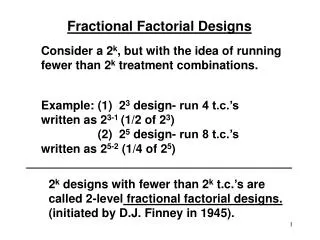
Fractional Factorial Designs. Consider a 2 k , but with the idea of running fewer than 2 k treatment combinations. Example: (1) 2 3 design- run 4 t.c.’s written as 2 3-1 (1/2 of 2 3 ) (2) 2 5 design- run 8 t.c.’s written as 2 5-2 (1/4 of 2 5 ).

Fractional Factorial Designs
E N D
Presentation Transcript
Fractional Factorial Designs Consider a 2k, but with the idea of running fewer than 2k treatment combinations. Example: (1) 23 design- run 4 t.c.’s written as 23-1 (1/2 of 23) (2) 25 design- run 8 t.c.’s written as 25-2 (1/4 of 25) 2k designs with fewer than 2k t.c.’s are called 2-level fractional factorial designs. (initiated by D.J. Finney in 1945).
Example: Run 4 of the 8 t.c.’s in 23: a, b, c, abc It is clear that from the(se) 4 t.c.’s, we cannot estimate the 7 effects (A, B, AB, C, AC, BC, ABC) present in any 23 design, since each estimate uses (all) 8 t.c.’s. What can be estimated from these 4 t.c.’s?
4A = -1 + a - b + ab - c +ac - bc + abc 4BC= 1 + a - b - ab - c - ac + bc + abc Consider (4A + 4BC)= 2(a - b - c + abc) or 2(A + BC)= a - b - c + abc overall: 2(A + BC)= a - b - c + abc 2(B + AC)= -a + b - c + abc 2(C + AB)= -a - b + c + abc In each case, the 4 t.c.’s NOT run cancel out. Note: 4ABC=(a+b+c+abc)-(1+ab+ac+bc) cannot be estimated.
Had we run the other 4 t.c.’s: 1, ab, ac, bc, We would be able to estimate A - BC B - AC C - AB (generally no better or worse than with + signs) NOTE: If you “know” (i.e., are willing to assume) that all interactions=0, then you can say either (1) you get 3 factors for “the price” of 2. (2) you get 3 factors at “1/2 price.”
Suppose we run these 4: 1, ab, c, abc; We would then estimate A + B C+ ABC AC + BC two main effects together usually less desirable } In each case, we “Lose” 1 effect completely, and get the other 6 in 3 pairs of two effects. { members of the pair are CONFOUNDED members of the pair are ALIASED
With 4 t.c.’s, one should expect to get only 3 “estimates” (or “alias pairs”) - NOT unrelated to “degrees of freedom being one fewer than # of data points” or “with c columns, we get (c-1) df.” In any event, clearly, there are BETTER and WORSE sets of 4 t.c.’s out of a 23. (Better & worse 23-1 designs)
Consider a 24-1 with t.c.’s 1, ab, ac, bc, ad, bd, cd, abcd A+BCD B+ACD C+ABD AB+CD AC+BD BC+AD D +ABC Can estimate: - 8 t.c.’s - Lose 1 effect - Estimate other 14 in 7 alias pairs of 2 Note:
Prospect in fractional factorial designs is attractive if in some or all alias pairs one of the effects is KNOWN. This usually means “thought to be zero.”
“Clean” estimates of the remaining member of the pair can then be made. For those who believe, by conviction or via selected empirical evidence, that the world is relatively simple, 3 and higher order interactions (such as ABC, ABCD, etc.) may be announced as zero in advance of the inquiry. In this case, in the 24-1 above, all main effects are CLEAN. Without any such belief, fractional factorials are of uncertain value. After all, you could get A + BCD =0, yet A could be large +, BCD large -; or the reverse; or both zero.
Despite these reservations fractional factorials are almost inevitable in a many factor situation. It is generally better to study 5 factors with a quarter replicate (25-2= 8) than 3 factors completely (23=8). Whatever else the real world is, it’s Multi-factored. The best way to learn “how” is to work (and discuss) some examples:
Example: 25-1: A, B, C, D, E Step 1: In a 2k-p, we must “lose” 2p-1. Here we lose 1. Choose the effect to lose. Write it as a “Defining relation” or “Defining contrast.” I = ABDE (in the plus-minus table) Step 2: Find the resulting alias pairs: *A=BDE AB=DE ABC=CDE B=ADE AC=4 BCD=ACE C=ABCDEAD=BE BCE=ACD D=ABE AE=BD E=ABD BC=4 CD=4 CE=4 - lose 1 -other 30 in 15 alias pairs of 2 -run 16 t.c.’s 15 estimates { *AxABDE=BDE
See if they’re (collectively) acceptable. Another option (among many others): I = ABCDE (in the plus-minus table) A=4 AB=3 B=4 AC=3 C=4 AD=3 D=4 AE=3 E=4 BC=3 BD=3 BE=3 CD=3 CE=3 DE=3 4: 4 way interaction; 3: 3 way interaction. Assume we choose I = ABDE
Next Step: Find the 2 blocks using ABDE as the confounded effect. I II 1c a ac ab abc b bc de cde ade acde abde abcde bde bcde ad acd d cd bd bcd abd abcd ae ace e ce be bce abe abce { Same process as a Confounding Scheme • Which block to run if I = ABDE (ABDE = “+”)?
Example 2: In a 25, there are 31 effects; with 8 runs, there are 7 df & 7 estimates available 25-2A, B, C, D, E { Must “Lose” 3; other 28 in 7 alias groups of 4
Choose the 3: Like in confounding schemes, 3rd must be product of first 2: I = ABC = BCDE = ADE A = BC = 5 = DE B = AC = 3 = 4 C = AB = 3 = 4 D = 4 = 3 = AE E = 4 = 3 = AD BD = 3 = CE = 3 BE = 3 = CD = 3 Find alias groups: Assume we use this design.
Let’s find the 4 blocks using ABC , BCDE , ADE as confounded effects 1 2 3 4 1 a b d abd bd ad ab bc abc c bcd acd cd abcd ac de ade bde e abe be ae abde bcde abcde cde bce ace ce abce acde • Which block should we run if I=ABC=BCDE=ADE?
Block 1: (in the plus-minus table) • the sign for ABC = “-” • the sign for BCDE = “+” • the sign for ADE = “-” } Defining relation is: I = -ABC = BCDE = -ADE Exercise: find the defining relations for the other blocks.
Analysis 2k-p Design using MINITAB • Create factorial design: • Stat>> DOE>> Factorial • >> Create Factorial Design • Input data values. • Analyze data: • Stat>> DOE>> Factorial • >> Analyze Factorial Design
A B C D rate-1 -1 -1 -1 45 1 -1 -1 1 100-1 1 -1 1 45 1 1 -1 -1 65-1 -1 1 1 75 1 -1 1 -1 60-1 1 1 -1 80 1 1 1 1 96 Example: 24-1 withdefining relation I=ABCD.
Analysis of Variance for rate (coded units) Source DF Seq SS Adj SS Adj MS F Main Effects 4 1663 1663 415.7 * 2-Way Interactions 3 1408 1408 469.5 * Residual Error 0 0 0 0.0 Total 7 3071
Fractional Factorial Fit: rate versus A, B, C, D Estimated Effects and Coefficients for rate (coded units) Term Effect Coef Constant 70.750 A 19.000 9.500 B 1.500 0.750 C 14.000 7.000 D 16.500 8.250 A*B -1.000 -0.500 A*C -18.500 -9.250 A*D 19.000 9.500
Alias StructureI + A*B*C*DA + B*C*DB + A*C*DC + A*B*DD + A*B*CA*B + C*DA*C + B*DA*D + B*C
Fractional Factorial Fit: rate versus A, C, D Estimated Effects and Coefficients for rate (coded units) Term Effect Coef SE Coef T P Constant 70.750 0.6374 111.00 0.000 A 19.000 9.500 0.6374 14.90 0.004 C 14.000 7.000 0.6374 10.98 0.008 D 16.500 8.250 0.6374 12.94 0.006 A*C -18.500 -9.250 0.6374 -14.51 0.005 A*D 19.000 9.500 0.6374 14.90 0.004 Analysis of Variance for rate (coded units) Source DF Seq SS Adj SS Adj MS F P Main Effects 3 1658.50 1658.50 552.833 170.10 0.006 2-Way Interactions 2 1406.50 1406.50 703.250 216.38 0.005 Residual Error 2 6.50 6.50 3.250 Total 7 3071.50 { We should also include alias structure like A(+BCD) for all terms.
From S.A.S: 1) 23 factorial (3 replicates for each of 8 cols): A L H Factor B Factor B L H L H 8,10, 24,28, 16,16, 28,18, 18 20 19 23 19,16 27,16, 16,25, 30,23, 16 17 22 25 L H C
Source DF Sum of Squares Mean Square Fvalue PR>F Model 7 432.0000000 61.71428571 3.38 0.0206 Error 16 292.0000000 18.25000000 Corr. Total 23 724.0000000 Source DF Type I SS F Value PR>F DF PR>F A 1 73.50000000 4.03 0.0620 1 0.0620 B 1 253.50000000 13.89 0.0018 1 0.0018 C 1 24.00000000 1.32 0.2683 1 0.2683 A*B 1 6.00000000 0.33 0.5744 1 0.5744 A*C 1 13.50000000 0.74 0.4025 1 0.4025 B*C 1 37.50000000 2.05 0.1710 1 0.1710 A*B*C 1 24.00000000 1.32 0.2683 1 0.2683 “p-values”
A AL AH A Low A High BL BH BL BH 36 69 72 51 60 63 51 78 BL BH BL BH 36 72 51 69 51 60 63 78 L CL CH D D DL DH CL CH H 2) 24-1
Source DF Sum of Squares Mean Square Fval Model 7 1296.0000000 185.14285714 Error 0 0.0000000 0.00000000 Corr. Total 7 1296.0000000 Source DF Type I SS F Value PR>F DF A + BCD 1 220.50000000 . . 1 B + ACD 1 760.50000000 . . 1 C + ABD 1 72.00000000 . . 1 A*B + CD 1 18.00000000 . . 1 A*C + BD 1 112.50000000 . . 1 B*C + AD 1 40.50000000 . . 1 A*B*C + D 1 72.00000000 . . 1
Real World Example of 28-2: Level FactorLH A Geography E W B Volume Cat. L H C Price Cat. L H D Seasonality NO YES E Shelf Space Normal Double F Price Normal 20% cut G ADV None Normal(IF) H Loc. Q Normal Prime Product Attributes { { Managerial Decision Variables
- E, F, G, H important - B, C, D main effects, but not important - A “less” important - XY,X= B, C, D very important Y= E, F, G, H -EF,EG,EH,FG,FH,GH very important - all > 3fi’s = 0, except EFG, EFH, EGH, FGH
I = BCD = ABEFGH = ACDEFGH Did objectives get met? A = 4 = 5 = 6 E,F,G,H = 4 = 5 = 6 (XY) BE = 3 = 4 = 7 .... DE,CE = 3 = 6 = 5 ... EF = 5 = 4 = 5 ... EFG = 6 = 3 = 4 Results:
An alternative: I = ABCD = ABEFGH = CDEFGH A = 3 = 5 = 7 E,F,G,H = 5 = 5 = 5 (XY) BE = 4 = 4 = 6 .... DE,CE = 4 = 6 = 4 ... EF = 6 = 4 = 4 ... EFG = 7 = 3 = 3
Minimum Detectable Effects in 2k-pWhen we testfor significance of an effect, we can also determine the power of the test.H0: A = 0Hl: A not = 0
By looking at power tables, we can determine the power of the test, by specifying s, and, essentially, (what reduces to) D, the true value of the A effect (since D = [true A - 0], = true A).Here, we look at the issue from an opposite (of sorts) perspective:Given a value of a, and for a given value of b (or power = 1-b), along with N and n,N = r • 2k-p = # of data pointsn = degrees of freedom for error term,
We can determine the “MDE,” the Minimum Detectable Effect (i.e., the minimum detectable D, so that the a and 1-b are achieved). The results are expressed in “s units,” since we don’t know s. Note: if r = 1 (no replication), there may be few (or even no) df left for error. The tables that follow assume that there are at least 3 df for an error estimate.First, a table of df, assuming that all main effects and as many 2fi’s as possible are cleanly estimated. (All 3fi’s and higher are assumed zero).
* 23 with 8 runs complete factorial 1 df for error (ABC)** 23 replicated twice 1 + 8 (for repl.) 9 df for error***25-1 replicated twice all 15 alias rows have mains or 2fi’s, only 16 df for error (replication)*** 25 no replication there will be 16 “3fi’s or higher” effects 16 df for error TABLES ON NEXT PAGES ASSUME DF OF THIS PAGE
TABLES 11.33 – 11.36 Of course, these tables can be used either1) find MDE, given a, 1-b, or2) find power, given MDE [required] and a.
Ex 1: 25-2, main effects and some 2fi’sa) a = .05, 1-b=.90, [b = .10] MDE = 3.5s (not good!!- effect must be very large to be detectable)b) Do a 25-1, 16 runs, with a = .05, 1-b=.90, [b=.10] MDE = 2.5s (not as bad!)Maybe settle for 1-b=.75, [b=.25] MDE = 2.0s
Ex 2:27, unreplicated, = 128 runsa = .01, 1-b=.99, [b=.01] MDE = .88s(e.g., if s estimate = .3 microns, MDE = .264 microns)Ex 3: 27-2, unreplicated, = 32 runsa = .05, 1-b=.95, [b=.05] MDE = 1.5s