Chapter 8 Two-Level Fractional Factorial Designs
500 likes | 1.16k Vues
Chapter 8 Two-Level Fractional Factorial Designs. 8.1 Introduction. The number of factors becomes large enough to be “interesting”, the size of the designs grows very quickly

Chapter 8 Two-Level Fractional Factorial Designs
E N D
Presentation Transcript
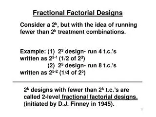
8.1 Introduction • The number of factors becomes large enough to be “interesting”, the size of the designs grows very quickly • After assuming some high-order interactions are negligible, we only need to run a fraction of the complete factorial design to obtain the information for the main effects and low-order interactions • Fractional factorial designs • Screening experiments: many factors are considered and the objective is to identify those factors that have large effects.
Three key ideas: • The sparsity of effects principle • There may be lots of factors, but few are important • System is dominated by main effects, low-order interactions • The projection property • Every fractional factorial contains full factorials in fewer factors • Sequential experimentation • Can add runs to a fractional factorial to resolve difficulties (or ambiguities) in interpretation
8.2 The One-half Fraction of the 2k Design • Consider three factor and each factor has two levels. • A one-half fraction of 23 design is called a 23-1 design
In this example, ABC is called the generator of this fraction (only + in ABC column). Sometimes we refer a generator (e.g. ABC) as a word. • The defining relation: I = ABC • Estimate the effects: • A = BC, B = AC, C = AB
Aliases: • Aliases can be found from the definingrelationI = ABC by multiplication: AI = A(ABC) = A2BC = BC BI =B(ABC) = AC CI = C(ABC) = AB • Principal fraction: I = ABC
The Alternate Fraction of the 23-1 design: I = - ABC • When we estimate A, B and C using this design, we are really estimating A – BC, B – AC, and C – AB, i.e. • Both designs belong to the same family, defined by I = ± ABC • Suppose that after running the principal fraction, the alternate fraction was also run • The two groups of runs can be combined to form a full factorial – an example of sequential experimentation
The de-aliased estimates of all effects by analyzing the eight runs as a full 23 design in two blocks. Hence • Design resolution: A design is of resolution R if no p-factor effect is aliased with another effect containing less than R – p factors. • The one-half fraction of the 23 design with I = ABC is a design
Resolution III Designs: • me = 2fi • Example: A 23-1 design with I = ABC • Resolution IV Designs: • 2fi = 2fi • Example: A 24-1 design with I = ABCD • Resolution V Designs: • 2fi = 3fi • Example: A 25-1 design with I = ABCDE • In general, the resolution of a two-level fractional factorial design is the smallest number of letters in any word in the defining relation.
The higher the resolution, the less restrictive the assumptions that are required regarding which interactions are negligible to obtain a unique interpretation of the data. • Constructing one-half fraction: • Write down a full 2k-1 factorial design • Add the kth factor by identifying its plus and minus levels with the signs of ABC…(K – 1) • K = ABC…(K – 1) => I = ABC…K • Another way is to partition the runs into two blocks with the highest-order interaction ABC…K confounded.
Any fractional factorial design of resolution R contains complete factorial designs in any subset of R – 1 factors. • A one-half fraction will project into a full factorial in any k – 1 of the original factors
Example 8.1: • Example 6.2: A, C, D, AC and AD are important. • Use 24-1 design with I = ABCD
This design is the principal fraction, I = ABCD • Using the defining relation, • A = BCD, B=ACD, C=ABD, D=ABC • AB=CD, AC=BD, BC=AD
A, C and D are large. • Since A, C and D are important factors, the significant interactions are most likely AC and AD. • Project this one-half design into a single replicate of the 23 design in factors, A, C and D. (see Figure 8.4 and Page 296)
Example 8.2: • 5 factors • Use 25-1 design with I = ABCDE (Table 8.5) • Every main effect is aliased with four-factor interaction, and two-factor interaction is aliased with three-factor interaction. • Table 8.6 (Page 298) • Figure 8.6: the normal probability plot of the effect estimates • A, B, C and AB are important • Table 8.7: ANOVA table • Residual Analysis • Collapse into two replicates of a 23 design
Sequences of fractional factorial: Both one-half fractions represent blocks of the complete design with the highest-order interaction confounded with blocks.
Example 8.3: • Reconsider Example 8.1 • Run the alternate fraction with I = – ABCD • Estimates of effects • Confirmation experiment
8.3 The One-Quarter Fraction of the 2k Design • A one-quarter fraction of the 2k design is called a 2k-2 fractional factorial design • Construction: • Write down a full factorial in k – 2 factors • Add two columns with appropriately chosen interactions involving the first k – 2 factors • Two generators, P and Q • I = P and I = Q are called the generating relations for the design • All four fractions are the family.
The complete defining relation: I = P = Q = PQ • P, Q and PQ are called words. • Each effect has three aliases • Aone-quarter fraction of the 26-2 with I = ABCE and I = BCDF. The complete defining relation is I = ABCE = BCDF = ADEF
Another way to construct such design is to derive the four blocks of the 26 design with ABCE and BCDF confounded , and then choose the block with treatment combination that are + on ABCE and BCDF • The 26-2 design with I = ABCE and I = BCDF is the principal fraction. • Three alternate fractions: • I = ABCE and I = - BCDF • I = -ABCE and I = BCDF • I = - ABCE and I = -BCDF
This fractional factorial will project into • A single replicate of a 24 design in any subset of four factors that is not a word in the defining relation. • A replicate one-half fraction of a 24 in any subset of four factors that is a word in the defining relation. • In general, any 2k-2 fractional factorial design can be collapsed into either a full factorial or a fractional factorial in some subset of r ≦ k –2 of the original factors.
Example 8.4: • Injection molding process with six factors • Design table (see Table 8.10) • The effect estimates, sum of squares, and regression coefficients are in Table 8.11 • Normal probability plot of the effects • A, B, and AB are important effects. • Residual Analysis (Pages 307-309)
8.4 The General 2k-p Fractional Factorial Design • A 1/ 2p fraction of the 2k design • Need p independent generators, and there are 2p –p – 1 generalized interactions • Each effect has 2p – 1 aliases. • A reasonable criterion: the highest possible resolution, and less aliasing • Minimum aberration design: minimize the number of words in the defining relation that are of minimum length.
Minimizing aberration of resolution R ensures that a design has the minimum # of main effects aliased with interactions of order R – 1, the minimum # of two-factor interactions aliased with interactions of order R – 2, …. • Table 8.14
Example 8.5 • Estimate all main effects and get some insight regarding the two-factor interactions. • Three-factor and higher interactions are negligible. • designs in Table 8-14 • 16-run design: main effects are aliased with three-factor interactions and two-factor interactions are aliased with two-factor interactions • 32-run design: all main effects and 15 of 21 two-factor interactions
Analysis of 2k-p Fractional Factorials: • For the ith effect: • Projection of the 2k-p Fractional Factorials • Project into any subset of r ≦ k – p of the original factors: a full factorial or a fractional factorial (if the subsets of factors are appearing as words in the complete defining relation.) • Very useful in screening experiments • For example 16-run design: Choose any four of seven factors. Then 7 of 35 subsets are appearing in complete defining relations.
Blocking Fractional Factorial: • Appendix Table XII • Consider the fractional factorial design with I = ABCE = BCDF = ADEF. Select ABD (and its aliases) to be confounded with blocks. (see Figure 8.18) • Example 8.6 • There are 8 factors • Four blocks • Effect estimates and sum of squares (Table 8.17) • Normal probability plot of the effect estimates (see Figure 8.19)
A, B and AD + BG are important effects • ANOVA table for the model with A, B, D and AD (see Table 8.18) • Residual Analysis (Figure 8.20) • The best combination of operating conditions: A –, B + and D –
8.5 Resolution III Designs • Designs with main effects aliased with two-factor interactions • A saturated design has k = N – 1 factors, where N is the number of runs. • For example: 4 runs for up to 3 factors, 8 runs for up to 7 factors, 16 runs for up to 15 factors • In Section 8.2, there is an example, design. • Another example is shown in Table 8.19: design I = ABD = ACE = BCF = ABCG = BCDE = ACDF = CDG = ABEF = BEG = AFG = DEF = ADEG = CEFG = BDFG = ABCDEFG
This design is a one-sixteenth fraction, and a principal fraction. I = ABD = ACE = BCF = ABCG = BCDE = ACDF = CDG = ABEF = BEG= AFG = DEF = ADEG = CEFG = BDFG = ABCDEFG • Each effect has 15 aliases.
Assume that three-factor and higher interactions are negligible. • The saturated design in Table 8.19 can be used to obtain resolution III designs for studying fewer than 7 factors in 8 runs. For example, for 6 factors in 8 runs, drop any one column in Table 8.19 (see Table 8.20)
When d factors are dropped , the new defining relation is obtained as those words in the original defining relation that do not contain any dropped letters. • If we drop B, D, F and G, then the treatment combinations of columns A, C, and E correspond to two replicates of a 23 design.
Sequential assembly of fractions to separate aliased effects: • Fold over of the original design • Switching the signs in one column provides estimates of that factor and all of its two-factor interactions • Switching the signs in all columns dealiases all main effects from their two-factor interaction alias chains – called a full fold-over
Example 8.7 • Seven factors to study eye focus time • Run design (see Table 8.21) • Three large effects • Projection? • The second fraction is run with all the signs reversed • B, D and BD are important effects
The defining relation for a fold-over design • Each separate fraction has L + U words used as generators. • L: like sign • U: unlike sign • The defining relation of the combining designs is the L words of like sign and the U – 1 words consisting of independent even products of the words of unlike sign. • Be careful – these rules only work for Resolution III designs
Plackett-Burman Designs • These are a different class of resolution III design • Two-level fractional factorial designs for studying k = N – 1 factors in N runs, where N = 4 n • N = 4, 8, 12, 16, 20, 24, 28, 32, 36, 40, … • The designs where N = 12, 20, 24, etc. are called nongeometric PB designs • Construction: • N = 12, 20, 24 and 36 (Table 8.24) • N = 28 (Table 8.23)
The alias structure is complex in the PB designs • For example, with N = 12 and k = 11, every main effect is aliased with every 2FI not involving itself • Every 2FI alias chain has 45 terms • Partial aliasing can greatly complicate interpretation • Interactions can be particularly disruptive • Use very, very carefully (maybe never)
Projection: Consider the 12-run PB design • 3 replicates of a full 22 design • A full 23 design + a design • Projection into 4 factors is not a balanced design • Projectivity 3: collapse into a full fractional in any subset of three factors.
Example 8.8: • Use a set of simulated data and the 11 factors, 12-run design • Assume A, B, D, AB, and AD are important factors • Table 8.25 is a 12-run PB design • Effect estimates are shown in Table 8.26 • From this table, A, B, C, D, E, J, and K are important factors. • Interaction? (due to the complex alias structure) • Folding over the design • Resolve main effects but still leave the uncertain about interaction effects.
8.6 Resolution IV and V Designs • Resolution IV: if three-factor and higher interactions are negligible, the main effects may be estimated directly • Minimal design: Resolution IV design with 2k runs • Construction: The process of fold over a design (see Table 8.27)
Fold over resolution IV designs: (Montgomery and Runger, 1996) • Break as many two-factor interactions alias chains as possible • Break the two-factor interactions on a specific alias chain • Break the two-factor interactions involving a specific factor • For the second fraction, the sign is reversed on every design generators that has an even number of letters
Resolution V designs: main effects and the two-factor interactions do not alias with the other main effects and two-factor interactions.