Download

1 / 27
270 likes | 323 Vues
Understand when to use and avoid the Two-Factor Design, its model, assumptions, computational steps, example calculations, error estimation, allocation of variation, ANOVA analysis, interpretation of results, and visual tests.

E N D
Two-FactorFull Factorial Designs Andy Wang CIS 5930 Computer Systems Performance Analysis
Two-Factor Design Without Replications • Used when only two parameters, but multiple levels for each • Test all combinations of levels of the two parameters • One replication per combination • For factors A and B with a and b levels, ab experiments required
When to Use This Design? • System has two important factors • Factors are categorical • More than two levels for at least one factor • Examples: • Performance of different CPUs under different workloads • Characteristics of different compilers for different benchmarks • Effects of different reconciliation topologies and workloads on a replicated file system
When to Avoid This Design? • Systems with more than two important factors • Use general factorial design • Non-categorical variables • Use regression • Only two levels • Use 22 designs
Model For This Design • yij is observation • m is mean response • j is effect of factor A at level j • i is effect of factor B at level i • eij is error term • Sums of j’s and i’s are both zero
Assumptions of the Model • Factors are additive • Errors are additive • Typical assumptions about errors: • Distributed independently of factor levels • Normally distributed • Remember to check these assumptions!
Computing Effects • Need to figure out , j, and i • Arrange observations in two-dimensional matrix • b rows, a columns • Compute effects such that error has zero mean • Sum of error terms across all rows and columns is zero
Two-Factor Full Factorial Example • Want to expand functionality of a file system to allow automatic compression • Examine three choices: • Library substitution of file system calls • New VFS • Stackable layers • Three different benchmarks • Metric: response time
Data for Example Library VFS Layers Compilation Benchmark 94.3 89.5 96.2 Email Benchmark 224.9 231.8 247.2 Web Server Benchmark 733.5 702.1 797.4
Computing • Averaging the jth column, • By assumption, error terms add to zero • Also, the j’s add to zero, so • Averaging rows produces • Averaging everything produces
Calculating Parameters for the Example • = grand mean = 357.4 • j = (-6.5, -16.3, 22.8) • i = (-264.1, -122.8, 386.9) • So, for example, the model predicts that the email benchmark using a special-purpose VFS will take 357.4 - 16.3 -122.8 = 218.3 seconds
EstimatingExperimental Errors • Similar to estimation of errors in previous designs • Take difference between model’s predictions and observations • Calculate Sum of Squared Errors • Then allocate variation
Allocating Variation • Use same kind of procedure as on other models • SSY = SS0 + SSA + SSB + SSE • SST = SSY - SS0 • Can then divide total variation between SSA, SSB, and SSE
Calculating SS0, SSA, SSB • Recall that a and b are number of levels for the factors
Allocation of Variationfor Example • SSE = 2512 • SSY = 1,858,390 • SS0 = 1,149,827 • SSA = 2489 • SSB = 703,561 • SST = 708,562 • Percent variation due to A: 0.35% • Percent variation due to B: 99.3% • Percent variation due to errors: 0.35%
Analysis of Variation • Again, similar to previous models, with slight modifications • As before, use an ANOVA procedure • Need extra row for second factor • Minor changes in degrees of freedom • End steps are the same • Compare F-computed to F-table • Compare for each factor
Analysis of Variation for Our Example • MSE = SSE/[(a-1)(b-1)] = 2512/[(2)(2)] = 628 • MSA = SSA/(a-1) = 2489/2 = 1244 • MSB = SSB/(b-1) = 703,561/2 = 351,780 • F-computed for A = MSA/MSE = 1.98 • F-computed for B = MSB/MSE = 560 • 95% F-table value for A & B is 6.94 • So A is not significant, but B is
Checking Our Resultswith Visual Tests • As always, check if assumptions made in the analysis are correct • Use residuals vs. predicted and quantile-quantile plots
What Does the Chart Reveal? • Do we or don’t we see a trend in errors? • Clearly they’re higher at highest level of the predictors • But is that alone enough to call a trend? • Perhaps not, but we should take a close look at both factors to see if there’s reason to look further • Maybe take results with a grain of salt
Confidence Intervalsfor Effects • Need to determine standard deviation for data as a whole • Then can derive standard deviations for effects • Use different degrees of freedom for each • Complete table in Jain, pg. 351
Standard Deviationsfor Example • se = sqrt(MSE) = 25.0 • Standard deviation of : • Standard deviation of j - • Standard deviation of i -
Calculating Confidence Intervals for Example • Only file system alternatives shown here • Use 95% level, 4 degrees of freedom • CI for library solution: (-39,26) • CI for VFS solution: (-49,16) • CI for layered solution: (-10,55) • So none of the solutions are significantly different than mean at 95%
Looking a Little Closer • Do zero CI’s mean that none of the alternatives for adding functionality are different? • Use contrasts to check (see section 20.7) • T-test should work as well