Download
1 / 9
100 likes | 268 Vues
Inference About Slope of a Regression Line. AP Stats Chapter 14. Some New Variables. Recall the formula for the LSRL: Where a was the y – intercept and b was the slope. For inference: Β is the population slope/true slope α is the population intercept/true intercept

E N D
Inference About Slope of a Regression Line AP Stats Chapter 14
Some New Variables • Recall the formula for the LSRL: • Where a was the y – intercept and b was the slope. • For inference: • Β is the population slope/true slope • α is the population intercept/true intercept • We will be testing the value of the slope.
Inference for Slope • Goal: to estimate the true slope β. • Assumptions: (to add to your cheat sheet) • Scatter plot is linear (check if needed). • Errors are independent( no pattern in the residual plot). • Variability of errors is constant (residual plot has a consistent spread). • Errors have a normal model (normal probability plot is reasonably straight.) • Yeah, it is a lot to remember!
Confidence Intervals • Formula: • Where • HOLD ON!! Don’t freak out! • The good news is that most of this is just from a computer print out or your calculator. • We will deal with that in a minute.
Confidence Intervals • New Degree of Freedom: df= n-2 • Because we are now dealing with two different variables. • Let’s do through an example with PANIC. • Turn to page 762 please. • We are looking for a 95% confidence interval for the true slope for ddays.
Confidence Intervals • Let’s Panic… • P = parameter of interest is β. • A = we are going to say that we are OK because we don’t have the exact data to check. (we will do another later.) • N = Confidence interval for regression slope. • I = Look at the computer printout… • .1890±(2.145)(.004934) • .1890±.0106 • .1784 to .1996 • C = We are 95% confident that the true average increase in usage associated with a 1 dday increase is between .1784 and .1996 cubic feet.
Hypothesis Test • Hypotheses: • Ho: β = 0 • Because if x doesn’t predict y at all, then y would not change. That would result in a horizontal line with a slope of zero! • Ha: β<,> or ≠ 0 • Test Stat: • P- Value: find on Table C (t – score) • Conclusions: Need to interpret what the slope is saying in context of the problem.
Hypothesis Test • Let’s take a look at pg. 761 #2… • P = parameter of interest is β • H = Ho: β=0 Ha: β > 0 (why?) • A = • Linear relationship – let’s check the scatter plot. • Errors independent - let’s check the residual plot • Variability constant - residuals again. • Errors normal – let’s check NPP. • N = t – test for slope
Hypothesis Test • T = go to calculator… • T = 49. 658 with df = 5 • O = p-value = close to zero • M = Reject Ho. • S = There is evidence that the speed of a runner predicts the steps per second where as speed increases, so do steps per second.