Inference About Regression Coefficients
Inference About Regression Coefficients. BENDRIX.XLS. This is a continuation of the Bendrix manufacturing example from the previous chapter. As before, the response variable is Overhead and the explanatory variables are MachHrs and ProRuns. The data are contained in this file.

Inference About Regression Coefficients
E N D
Presentation Transcript
BENDRIX.XLS • This is a continuation of the Bendrix manufacturing example from the previous chapter. • As before, the response variable is Overhead and the explanatory variables are MachHrs and ProRuns. • The data are contained in this file. • What inferences can we make about the regression coefficients?
Multiple Regression Output • We obtain the output from using StatPro’s Multiple Regression procedure.
Multiple Regression Output -- continued • Regression coefficients estimate the true, but unobservable, population coefficients. • The standard error of bi indicates the accuracy of these point estimates. • For example, the effect on Overhead of a one-unit increase in MachHrs is 43.536. • We are 95% confident that the coefficient is between 36.357 to 50.715. Similar statements can be made for the coefficient of ProdRuns and the intercept term.
The Problem • We want to explain a person’s height by means of foot length. • The response variable is Height, and the explanatory variables are Right and Left, the length of the right foot and the left foot, respectively. • What can occur when we regress Height on both Right and Left?
Multicollinearity • The relationship between the explanatory variable X and the response variable Y is not always accurately reflected in the coefficient of X; it depends on which other X’s are included or not included in the equation. • This is especially true when there is a linear relationship between to or more explanatory variables, in which case we have multicollinearity. • By definition multicollinearity is the presence of a fairly strong linear relationship between two or more explanatory variables, and it can make estimation difficult.
Solution • Admittedly, there is no need to include both Right and Left in an equation for Height - either one would do - but we include both to make a point. • It is likely that there is a large correlation between height and foot size, so we would expect this regression equation to do a good job. • The R2 value will probably be large. But what about the coefficients of Right and Left? Here is a problem.
Solution -- continued • The coefficient of Right indicates that the right foot’s effect on Height in addition to the effect of the left foot. This additional effect is probably minimal. That is, after the effect of Left on Height has already been taken into account, the extra information provided by Right is probably minimal. But it goes the other way also. The extra effort of Left, in addition to that provided by Right, is probably minimal.
HEIGHT.XLS • To show what can happen numerically, we generated a hypothetical data set of heights and left and right foot lengths in this file. • We did this so that, except for random error, height is approximately 32 plus 3.2 times foot length (all expressed in inches). • As shown in the table to the right, the correlations between Height and either Right or Left in our data set are quite large, and the correlation between Right and Left is very close to 1.
Solution -- continued • The regression output when both Right and Left are entered in the equation for Height appears in this table.
Solution -- continued • This output tells a somewhat confusing story. • The multiple R and the corresponding R2 are about what we would expect, given the correlations between Height and either Right or Left. • In particular, the multiple R is close to the correlation between Height and either Right or Left. Also, the se value is quite good. It implies that predictions of height from this regression equation will typically be off by only about 2 inches.
Solution -- continued • However, the coefficients of Right and Left are not all what we might expect, given that we generated heights as approximately 32 plus 3.2 times foot length. • In fact, the coefficient of Left has the wrong sign - it is negative! • Besides this wrong sign, the tip-off that there is a problem is that the t-value of Left is quite small and the corresponding p-value is quite large.
Solution -- continued • Judging by this, we might conclude that Height and Left are either not related or are related negatively. But we know from the table of correlations that both of these are false. • In contrast, the coefficient of Right has the “correct” sign, and its t-value and associated p-value do imply statistical significance, at least at the 5% level. • However, this happened mostly by chance, slight changes in the data could change the results completely.
Solution -- continued • The problem is although both Right and Left are clearly related to Height, it is impossible for the least squares method to distinguish their separate effects. • Note that the regression equation does estimate the combined effect fairly well, the sum of the coefficients is 3.178 which is close to the coefficient of 3.2 we used to generate the data. • Therefore, the estimated equation will work well for predicting heights. It just does not have reliable estimates of the individual coefficients of Right and Left.
Solution -- continued • To see what happens when either Right or Left are excluded from the regression equation, we show the results of simple regression. • When Right is only variable in the equation, it becomesPredicted Height = 31.546 + 3.195Right • The R2 and se values are 81.6% and 2.005, and the t-value and p-value for the coefficient of Right are now 21.34 and 0.000 - very significant.
Solution -- continued • Similarly, when the Left is the only variable in the equation, it becomesPredicted Height = 31.526 + 3.197Left • The R2 and se values are 81.1% and 2.033, and the t-value and p-value for the coefficient of Left are 20.99 and 0.0000 - again very significant. • Clearly, both of these equations tell almost identical stories, and they are much easier to interpret than the equation with both Right and Left included.
CATALOGS1.XLS • This file contains data on 100 customers who purchased mail-order products from the HyTex Company in 1998. • Recall from Example 3.11 that HyTex is a direct marketer of stereo equipment, personal computers, and other electronic products. • HyTex advertises entirely by mailing catalogs to its customers, and all of its orders are taken over the telephone. • We want to estimate and interpret a regression equation for Spent98 based on all of these variables.
The Data • The company spends a great deal of money on its catalog mailings, and it wants to be sure that this is paying off in sales. • For each customer there are data on the following variables: • Age in years. • Gender: coded as 1 for males, 0 for females • OwnHome: coded as 1 if customer owns a home, 0 otherwise • Married: coded as 1 if customer is currently married, 0 otherwise
The Data -- continued • Close: coded as 1 if customers lives reasonably close to a shopping area that sells similar merchandise, 2 otherwise • Salary: combined annual salary of customer and spouse (if any) • Children: number of children living with customer • Customer97: coded as a 1 if customer purchased from HyTex during 1997, 0 otherwise • Spent97: total amount of purchase made from HyTex during 1997 • Catalogs: Number of catalogs sent to the customer in 1998 • Spent98: total amount of purchase made from HyTex during 1998
The Data -- continued • With this much data, 1000 observations, we can certainly afford to set aside part of the data set for validation. • Although any split could be used, let’s base the regression on the first 250 observations and use the other 750 for validation.
The Regression • We begin by entering all of the potential explanatory variables. • Our goal then is exclude variables that aren’t necessary, based on their t-values and p-values. To do this we follow the Guidelines for Including / Excluding Variables in a Regression Equation. • The regression output with all explanatory variables included is provided on the following slide.
Analysis • This output indicates a fairly good fit. The R2 value is 79.1% and se is about $424. • From the p-value column, we see that there are three variables, Age, Own_Home, and Married, that have p-values well above 0.05. • These are the obvious candidates for exclusion. It is often best to exclude one variable at a time starting with the variable with the highest p-value. • The regression output with all insignificant variables excluded is seen in the output on the next slide.
Interpretation of Final Regression Equation • The coefficient of Gender implies that an average male customer spent about $130 less than the average female customer. Similarly, an average customer living close to stores with this type of merchandise spent about $288 less than those customers living far form stores. • The coefficient of Salary implies that, on average, about 1.5 cents of every salary dollar was spent on HyTex merchandise.
Interpretation of Final Regression Equation -- continued • The coefficient of Children implies that $158 less was spent for every extra child living at home. • The Customer97 and Spent97 terms are somewhat more difficult to interpret. • First, both of these terms are 0 for customers who didn’t purchase from HyTEx in 1997. • For those that did the terms become -724 + 0.47Spent97 • The coefficient 0.47 implies that each extra dollar spent in 1997 can be expected to contribute an extra 47 cents in 1998.
Interpretation of Final Regression Equation -- continued • The median spender in 1997 spent about $900. So if we substitute this for Spent 97 we obtain -301. • Therefore, this “median” spender from 1997 can be expected to spend about $301 less in 1998 than the 1997 nonspender. • The coefficient of Catalog implies that each extra catalog can be expected to generate about $43 in extra spending.
Cautionary Notes • When we validate this final regression equation with the 750 customers, using the procedure from Section 11.7, we find R2 and se values of 75.7% and $485. • These aren’t bad. They show little deterioration from the values based on the original 250 customers. • We haven’t tried all possibilities yet. We haven’t tried nonlinear or interaction variables, nor have we looked at different coding schemes; we haven’t checked for nonconstant error variance or looked at potential effects of outliers.
BANK.XLS • Recall from Example 11.3 that the Fifth National Bank has 208 employees. • The data for these employees are stored in this file. • In the previous chapter we ran several regressions for Salary to see whether there is convincing evidence of salary discrimination against females. • We will continue this analysis here.
Analysis Overview • First, we will regress Salary versus the Female dummy, YrsExper, and the interactions between Female and YrsExper, labeled Fem_YrsExper. This will be the reduced equation. • Then we’ll see whether the JobGrade dummies Job_2 to Job_6 add anything significant to the reduced equation. If so, we will then see whether the interactions between the Female dummy and the JobGrade dummies, labeled Fem_Job2 to Fem_Job6, add anything significant to what we already have.
Analysis Overview -- continued • If so, we’ll finally see whether the education dummies Ed_2 to Ed_5 add anything significant to what we already have.
Solution • First, note that we created all of the dummies and interaction variables with StatPro’s Data Utilities procedures. • Also, note that we have used three sets of dummies, for gender, job grad and education level. • When we use these in a regression equation, the dummy for one category of each should always be excluded; it is the reference category. The reference categories we have used are “male”, job grade 1 and education level 1.
Solution -- continued • The output for the “smallest” equation using Female, YrsExper, and Fem_YrsExper as explanatory variables is shown here.
Solution -- continued • We’re off to a good start. These three variables already explain 63.9% of the variation of Salary. • The output for the next equation which adds the explanatory variables Job_2 to Job_6 is on the next slide. • This equation appears much better. For example R2 has increased to 81.1%. We check whether it is significantly better with the partialtest in rows 26-30.
Solution -- continued • The degrees of freedom in cell C28 is the same as the value in cell C12, the degrees of freedom for SSE. • Then we calculate the F-ratio in cell C29 with the formula =((Reduced!D12-D12)/C27)/E12 were Reduced!D12 refers to SSE for the reduced equation from the Reduced sheet. • Finally, we calculate the corresponding p-value in cell C30 with the formula =FDIST(C29,C27,C28). It is practically 0, so there is no doubt that the job grade dummies add significantly to the explanatory power of the equation.
Solution -- continued • Do the interactions between the Female dummy and the job dummies add anything more? • We again use the partial F test, but now the previous complete equation becomes the new reduced equation, and the equation that includes the new interaction terms becomes the new equation. • The output for this new complete equation is shown on the next slide. • We perform the partial F test in rows 31-35 as exactly as before. The formula in C34 is =((Complete!D12-D12)/C32)/E12.
Solution -- continued • Again the p-value is extremely small, so there is no doubt that the interaction terms add significantly to what we already had. • Finally, we add the education dummies. • The resulting output is shown on the next slide. We see how the terms reduced and complete are relative. • This output now corresponds to the complete equation, and the previous output corresponds to the reduced equation.
Solution -- continued • The formula in cell C38 for the F-ratio is now =((MoreComplete!D12-D12/C36)/E12. The R2 value increased from 84.0% to 84.7%. Also the p-value is not extremely small. • According to the partial F test, it is not quite enough to qualify for statistical significance at the 5% level. • Based on this evidence, there is not much to gain from including the education dummies in the equation, so we would probably elect to exclude them.
Concluding Comments • First, the partial test is the formal test of significance for an extra set of variables. Many users look only at the R2 and/or se values to check whether extra variables are doing a “good job”. • Second, if the partial F test shows that a block of variables is significant, it does not imply that each variable in this block is significant. Some of these values can have low t-values.
Concluding Comments -- continued • Third, producing all of these outputs and doing the partial F tests is a lot of work. Therefore, we included a “Block” option in StatPro to make life easier. To run the analysis in this example use StatPro/Regression analysis/Block menu item. After selecting Salary as the response variable, we see this dialog box.
Concluding Comments -- continued • We want four blocks of explanatory variables, and we want a given block to enter only if it passes the partial F test at the 5% level. In later dialog boxes we specify the explanatory variables. Once we have specified all this, the regression calculations are done in stages. The output from this appears on the next two slides. The output spans over two figures. Note that the output for Block 4 has been left off because it did not pass the F test at 5%.
Concluding Comments -- continued • Finally, we have concentrated on the partial F test and statistical significance in this example. We don’t want you to lose sight, however, of the bigger picture. Once we have decided on a “final” regression equation we need to analyze its implications for the problem at hand. • In this case the bank is interested in possible salary discrimination against females, so we should interpret this final equation in these terms. Our point is simply that you shouldn’t get so caught in the details of statistical significance that you lose sight of the original purpose of the analysis!