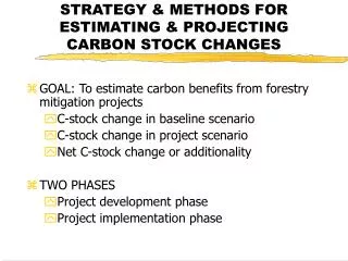
STRATEGY & METHODS FOR ESTIMATING & PROJECTING CARBON STOCK CHANGES

1. STRATEGY & METHODS FOR ESTIMATING & PROJECTING CARBON STOCK CHANGES • GOAL: To estimate carbon benefits from forestry mitigation projects • C-stock change in baseline scenario • C-stock change in project scenario • Net C-stock change or additionality • TWO PHASES • Project development phase • Project implementation phase • systems

2. Steps for Carbon inventory • Step 1: Definition of objectives, land use systems and area for estimating carbon benefits of a project • Step 2: Description of project activities and area • Step 3: Selection of C-pools and methods for measurement and monitoring the pools by selecting the parameters for each pool • Step 4: Definition of the project boundary and map preparation • Step 5: Stratification of the ecosystem and land use

3. Contd…………. • Step 6: Developing sampling design and strategy for biomass and soil carbon • Step 7: Laying plots in different land use systems • Step 8: Field measurements, data format and data recording • Step 9: Data analysis for biomass and soil carbon estimation • Step 10: Projecting C-stock changes using PROCOMAP model • Step 11:Reporting C-stocks for different pools under baseline and project scenario • Step 12: Reporting of incremental carbon benefits

4. Step-1: Objective; • i) Estimating C-stock changes in BSL & Project scenario • Step-2 & 3: Land use systems & project activities • Land use systems: Degraded forestland, farmland, village commons • Project activities: A&R- Natural regeneration, mixed-species forestry, plantation • Area under these categories

5. Step-4: Selection of carbon pools

6. Step 5: Selection of Methods

7. Step-6: Parameters to be measured

8. Project boundary and map

9. Step-8: Stratification of project area

10. Sampling at project development phase • Baseline scenario: • Degraded forestland • Degraded pasture land • Degraded farmland • Project scenario-Activities: • Natural regeneration • Different years (near by area) • Mixed species plantation • Different years (near by area) • Monoculture plantation • Different age (near by area) • Plots to be laid in all such land categories

11. Step-9: Sampling design & Strategy • METHOD: ‘Plot method’ / ‘Quadrat method’ • TYPE OF PLOT: Quadrat, circular, strip

12. Size & Number of Plots • Statistical approach: Based on estimates; variance of C-stock, cost of sampling and precision • Thumb rule; used most often • Sampling separately for trees, shrubs, herbs

13. Land use systems Trees Shrub Herb/Grass Soil Size of plot (m) No. of plots Size of plot (m) No. of plots Size of plot (m) No. of plots Size of plot (m) No. of plots Natural regeneration or Heterogenous vegetation 50 X 40 5 5 X 5 10 1 X 1 20 1 X 1 20 50 X 50 4 5 X 5 10 1 X 1 20 1 X 1 20 Plantations with homogenous vegetation or Uniform species distribution and density 50 X 20 or 40 X 25 5 5 X 5 8 1 X 1 16 1 X 1 16 Degraded forest or barren or fallow land 50 X 40 5 5 X 5 10 1 X 1 20 1 X 1 20 Examples of Number & Size of plots

14. Sampling sites at Project development phase • Baseline scenario- Land use systems • Degraded forestland • Degraded village commons • Farmland • Project activities • Teak regeneration; 5 or 10 or 15 yrs • Secondary forest regeneration; 5 or 12 or 20 yrs • Natural forest (old growth)

15. Step 10: Laying of plots in the field • I. Stratified Random Sampling • II. Systematic Sampling

16. Stratified Random Sampling • Involves locating the plots in the field in an unbiased way & suitable to both heterogeneous and homogenous vegetation • Sampling approach involves following steps: • Step 1: Stratify land use systems & project activity areas • Step 2: Prepare a grid map of the project area, demarcating each land use system or project activity. Size of the grid as small as feasible (say 50 m X 50 m) • Step 3: Give numbers to each grid • Step 4: Randomly pick the grid numbers, using random table or lottery system.

17. Contd…………….. • Step 5: Locate tree plots in the grids selected in the field with respect to some permanent visible land mark and mark the boundary of each tree plot or use GPS • Step 6: Prepare and store a map with all the details, including the location of sample plots marked on it. • Location of sample plots in the field; overlay the land use system map over the grid scale map • Using GIS & marking plots in the selected grids. GPS measurements of the corner points of plots must be recorded on the map for revisits

18. Systematic sampling • Employs a simple method of selecting every kth unit (grid) starting with a number chosen at random from 1 to N. • Step 1: Select the number of plots (quadrats) for the study (n), which have to be laid in the field for sampling, say for example n = 5 of 50 m X 40 m dimension • Step 2: Stratify the land use system into homogenous sub-strata • Step 3: Obtain a map showing the grids depicting each sampling stratum and estimate the total number of grids for each strata (N), say for example 200 grids with an area of 40 ha • Step 4: Calculate the sampling interval ‘k’ by using the following equation, • k = N/n where, k = sampling interval of grids or plots = 200/5 = 40

19. Contd…………... • Step 5: Draw a random number which is less than k (sampling interval for grid), say 25th grid • Step 6: Select and mark the first grid based on the random number selected • First sampling grid or plot number is 25 • Second sampling grid or plot = Sampling interval k (40) + first sampling grid (25) = 65th grid • Third sampling grid or plot = Sampling interval k (40) + second sampling grid (65) = 105th grid. • Similarly, the successive grids or plots will be systematically sampled, till the nth grid or plot (in the example 5th grid) is located.

20. Field measurements: Trees

21. GBH/DBH measurement

22. Field measurements: Shrubs

23. Woody litter including Fallen deadwood • Woody litter production • Standing woody litter • STEPS: STANDING WOODY LITTER • Step 1: Select and use the shrub plots marked in the field • Step 2: Select the peak month when the litter fall is maximum based on local experience • Step 3: Collect woody litter from all shrub plots and merge to one heap & estimate the fresh weight • Step 4: Take a sample of say 1 kg for dry weight estimation in the laboratory as % of fresh weight • Step 5: Estimate weight of dry woody litter per hectare using fresh and dry weight litter data and area of shrub plots.

24. Soil carbon • Soil carbon is the dominant C-pool in many projects • Soil carbon in top 15 & 30 cm • Collecting soil sample for carbon estimation involves the following steps: • Step 1: Select the plots marked for shrub biomass estimation, 8 to 10 plots • Step 2: Mark the mid-point of the 5mx5m shrub plot or any point randomly

25. Contd……... • Step 3: Using the soil agar, drill the soil to a depth of 0-15 cm and collect the sample. Repeat procedure for 15-30 cm depth. • Step 4: Merge soil samples of 0-15 cm from the two shrub plots of a tree plot. Remove plant debris. Collect about 0.5 kg of fresh soil into a plastic bag for laboratory analysis. Repeat for 15-30 cm soil depth.

26. Bulk density • Converting SOC concentration (in % terms) to tC/ha needs bulk density • Step 1: Select 1 shrub plot, out of 2 plots laid per tree plot • Step 2: Weigh an empty bottle & fill this with soil. Tap the bottle, keep filling the soil till the level reaches the brim. Mark the level of soil in the bottle. The compaction of the soil in the bottle may be comparable to what is present in the field • Step 3: Note down the weight of the bottle with the soil • Step 4: Empty the bottle and add water to the container till the marked level. Note down the volume of the water by pouring it in the measuring cylinder

27. Equations for SOC • Bulk density (g/cc) = (Weight of the soil in the bottle)/ (Volume of the water in the bottle) • Soil mass (t/ha) = [Area (10,000 m2) X Depth (0.3 m) X Bulk density X 103 grams/Kg]/(1000Kg/tonne) • SOC (tonne/ha) = (Soil mass in 0-30 cm) X SOC concentration (%)/100

28. Biomass estimation • AGB; i) Using biomass equations • Generic • Species specific • Based on: DBH, Height & Basal area • ii) Volume estimation of trees • iii) Harvest method; plantations • BGB; AGB X 0.26 • Litter; Stock at base-year and project-year • Carbon; Biomass X 0.5

29. Estimating Net Additional Incremental Carbon Benefit • Reporting incremental carbon benefits requires estimation and reporting of: • Net change in C-stock covering all C-pools in baseline scenario & project scenario • Estimation of leakage of carbon benefits • Incremental carbon benefit (in tC for the period selected) = (net change in C-stock in project scenario) - (net change in C-stock in baseline scenario) - (estimated leakage)

30. Contd…….. • Carbon benefits of the project = [(Total carbon stock at end of 5 years) – (Total carbon stock at year 0)] • Net incremental carbon benefits = (Estimates of carbon benefits under the project scenario) - (Baseline scenario carbon stock change) - (Leakage estimates)

31. Monitoring of C-stock changes • Adopt plot method • Select frequency of monitoring • AGB: 2 or 3 years • SOC: 5 years • Conduct field & Lab studies • Estimate C-stocks

32. Criteria for Selection of Project Site • Availability of multiple land categories • Community lands/Government lands • Open forest land • Farm land for afforestation • Forestland subjected to extensive extraction • Contiguous parcel (cluster of villages) with in a forest division or range • 10 to 30 villages • 5000 to 10,000 ha

33. Contd…….. • Potential for Community forestry/JFM • Case study - I • Potential for ‘Industry-farmers’ cooperative • Case study- II • Potential for high carbon sequestration growth rates - Initial phase • Soil status • Rainfall