Download

1 / 70
730 likes | 973 Vues
Chapter 3 Individual Demand Curves. Demand Functions. Knowing a person’s preferences and all the economic forces that affect choices allows a prediction of how much of each good a person would choose in the face of scarcity

E N D
Chapter 3 Individual Demand Curves
Demand Functions • Knowing a person’s preferences and all the economic forces that affect choices allows a prediction of how much of each good a person would choose in the face of scarcity • Summarizes this information in a demand function: a representation of how the quantity demanded depends on prices, income, and preferences.
Demand Function • Three elements determine quantity demanded: • Prices of X and Y • Income (I) • Person’s preferences for X and Y. • Preferences appear to the right of semicolon - assume that preferences do not change during analysis (i.e. it is static) {3.1}
Changes in Income • When income increases and prices remain the same, the quantity of each good purchased might increase. • Shown in Figure 3-1 where an increase in income shows as a shift of budget line outward from I1 to I2 to I3. • Slope of budget lines remain the same because prices have not changed .
FIGURE 3-1: Effect of Increasing Income on the Quantities of X and Y Chosen
FIGURE 3-1: Effect of Increasing Income on the Quantities of X and Y Chosen
FIGURE 3-1: Effect of Increasing Income on Quantities of X and Y Chosen Quantity of Y per week Y3 Y2 U3 U2 Y1 U1 I2 I3 I1 Quantity of X per week 0 X1 X2 X3
Changes in Income • Response to increased income: quantity of X purchased increases from X1 to X2 and X3 while the quantity purchased of Y also increases from Y1 to Y2 to Y3. • Income increases allow more consumption, and are reflected in an outward shift in the budget constraint. Allows an increase in overall utility.
Normal Goods & Inferior Goods • Normal good: bought in greater quantities as income increases • Inferior good: bought in smaller quantities as income increases.
FIGURE 3-2: Indifference Curve Map Showing Inferiority Quantity of Y per week Y1 U1 Quantity of Z per week I1 Z1 0
FIGURE 3-2: Indifference Curve Map Showing Inferiority Quantity of Y per week Y2 U2 Y1 U1 I2 I1 Quantity of Z per week Z2 Z1 0
FIGURE 3-2: Indifference Curve Map Showing Inferiority Quantity of Y per week Y3 U3 Y2 U2 Y1 U1 I1 I2 I3 Quantity of Z per week Z2 Z1 0 Z3
Changes in a Good’s Price • Change in the price of one good causes both slope and the intercept of the budget line to change. • Change in one good’s price creates a new utility-maximizing choice on another indifference curve with a different MRS. • Change in quantity demanded of good with price change
Substitution Effect • Part of the change in the quantity demanded for other goods is caused by the substitution of one good for another: called substitution effect • Movement along an indifference curve • Consumption has to change to equate MRS to the new price ratio of the two goods.
Income Effect • Price change creates difference in real purchasing power; consumers move to a new indifference curve consistent with their new purchasing power • Part of the change in the quantity demanded is caused by the change in real income: called income effect.
Substitution and Income Effects from a Fall in Price • Figure 3-3: when the price of good X falls, the budget line rotates out from the unchanged Y axis, such that the X intercept lies farther out - the consumer can now buy more X with lower price. • Flatter slope means that relative price of X to Y (PX/PY) has fallen.
FIGURE 3-3: Income and Substitution Effects of a Fall in Price Quantity of Y per week Y* U1 Quantity of X per week 0 X*
FIGURE 3-3: Income and Substitution Effects of a Fall in Price
FIGURE 3-3: Income and Substitution Effects of a Fall in Price
Figure 3-4: Relative Size of Substitution Effects Right Shoes Shell . A,B U1 I I’ I’ I U1 BP Left Shoes (a) Small Substitution Effect ’ (b) Large Substitution Effect
Substitution and Income Effects from an Increase in Price • Increase in PX will shift budget line in toward origin, as in Figure 3-5. • Substitution effect, holding “real” income constant: move on U2 from X*, Y* to point B • Because a higher price decreases purchasing power, movement from B to X**, Y** is the income effect
FIGURE 3-5: Income and Substitution Effects of an Increase in Price Quantity of Y per week U2 New budget constraint Y* Old budget constraint Quantity of X per week 0 X*
FIGURE 3-5: Income and Substitution Effects of an Increase in Price Quantity of Y per week U2 U1 B New budget constraint Y* Old budget constraint Quantity of X per week 0 XB X* Substitution effect
FIGURE 3-5: Income and Substitution Effects of an Increase in Price
Substitution and Income Effects for a Normal Good: Summary • Figures 3-3 and 3-5 show that substitution and income effects work in the same direction with a normal good. • When the price falls, both substitution and income effects result in more being purchased. • When price increases, both substitution and income effects result in less being purchased.
Substitution and Income Effects for a Normal Good: Summary • These effects provide a rationale for downward sloping demand curves. • Also help to determine steepness of demand curve • If either substitution or income effects are large, the change in quantity demanded will be large with a given price change.
Substitution and Income Effects for Inferior Goods • With an inferior good, the substitution and income effects work in opposite directions. • Substitution effect results in decreased consumption for price increases and increased consumption for price decreases.
FIGURE 3-6: Income and Substitution Effects for Inferior Good Quantity of Y per week Y* U2 Old budget constraint Quantity of X per week 0 X*
Substitution and Income Effects for Inferior Goods • For inferior goods, the income effect results in an increased consumption for a price increase, and decreased consumption for a price decrease. • Figure 3-6 shows income and substitution effects for an increase in PX. • Substitution effect, holding real income constant, appears as a move from X*, Y* to point B both on U2.
FIGURE 3-6: Income and Substitution Effects for Inferior Good Quantity of Y per week B New budget constraint Y* U2 Y** Old budget constraint U1 Quantity of X per week 0 X*
FIGURE 3-6: Income and Substitution Effects for Inferior Good Quantity of Y per week B New budget constraint Y* U2 Y** Old budget constraint U1 Quantity of X per week 0 X** X*
Substitution and Income Effects: Inferior Goods • Income effect reflects reduced purchasing power due to a price increase. • X is an inferior good: decreased income results in increased consumption of X - shown by a move from point B on U1 to a new utility maximizing point X**, Y** on U1.
Substitution and Income Effects for Inferior Goods • Since X** is less than X*, X price increase results in a decreased consumption of X. • Decreased consumption happens because the substitution effect, in this example, is bigger than the income effect. • Thus, if the substitution effect dominates, the demand curve is negatively sloped.
Giffen’s Paradox • If the income effect of price change for an inferior good is strong enough, the quantity demanded may change in same direction as the price change. • A situation in which an increase in a good’s price, leads people to consume more of the good is called Giffen’s paradox.
The Lump Sum Principle • “Lump-sum principle” holds that taxes imposed on general purchasing power will have smaller welfare costs than will taxes imposed on a narrow selection of commodities. • Consider Figure 3-7: an individual initially has I euros to spend, and chooses to consume X* and Y*, yielding U3 utility.
FIGURE 3-7: The Lump-Sum Principle Quantity of Y I Y* U3 Quantity of X per week X*
The Lump Sum Principle • A tax on only good X raises its price, resulting in a budget constraint I*, and consumption reduced to X1, Y1 and utility level U1. • A general income tax that generates the same total tax revenue is represented by the budget constraint I** that goes though X1, Y1.
FIGURE 3-7: The Lump-Sum Principle Quantity of Y I Y1 Y* I’ Y2 U3 U1 Quantity of X per week X1 X*
FIGURE 3-7: The Lump-Sum Principle Quantity of Y I Y1 Y* I’ I” Y2 U3 U2 U1 Quantity of X per week X1 X2 X*
The Lump Sum Principle • Intuitive explanation of lump-sum principle: a single-commodity tax affects consumers in two ways: • Reduces their purchasing power, • Directs consumption away from the good being taxed. • The lump-sum tax only has the first of these two effects.
Changes in the Price of Another Good • In a two-good economy, when the price of one good changes, it affects the demand for the other good. • Figure 3-3: an increase in the price of X (a normal good) caused both an income and substitution effect that caused a reduction in the quantity demanded of X.
Changes in the Price of Another Good • In addition, the substitution effect caused the demand to decrease for good Y as the consumer substituted good X for good Y. • To offset, the purchasing power increase brought about by a price decrease, causes an increase in the demand for good Y (also a normal good).
Changes in the Price of Another Good • In this case, the income effect had a dominant effect on good Y - consumption of Y increased due to the decrease in X’s price. • With flatter indifference curves as shown in Figure 3-8, the situation reverses. • Decrease in X’s price causes a decrease in the consumption of good Y, as before.
FIGURE 3-8: Effect on the Demand for Good Y of a Decrease in the Price of Good X Quantity of Y per week Old budget constraint Y* U1 Quantity of X per week 0 X*
FIGURE 3-8: Effect on the Demand for Good Y of a Decrease in the Price of Good X Quantity of Y per week Old budget constraint A Y* B New budget constraint U2 U1 Quantity of X per week 0 X*
FIGURE 3-8: Effect on the Demand for Good Y of a Decrease in the Price of Good X Quantity of Y per week Old budget constraint A Y* C Y** B New budget constraint U2 U1 Quantity of X per week 0 X* X**
Changes in the Price of Another Good – Substitutes & Complements • Here, the income effect is much smaller than the substitution effect, so the consumer ends up consuming less of good Y at Y** after a decrease in X’s price. • Thus, the effect of a change in the price of one good has an ambiguous effect on demand for the other good.
Construction of Individual Demand Curves • Individual demand curve: is a graphic representation between the price of a good and the quantity demanded by a consumer, holding all other factors (preferences, prices of other goods, and income) constant • Demand curves limit the study to the relationship between the quantity demanded and changes in the good’s price - a single good world
Construction of Individual Demand Curves • Panel a of Figure 3-9: an individual’s indifference curve map drawn using three different budget constraints - Px decreases • Decreasing prices: P’X, P”X, and P’’’X respectively • Individual’s utility maximizing choices of quantity of X: X’, X’, and X’’’ respectively