Decision-Making with A Strategic Emphasis
1.01k likes | 1.71k Vues
Chapter Eleven. Decision-Making with A Strategic Emphasis. Relevant Cost Analysis. A relevant cost is a future cost that differs between the decision alternatives Both characteristics must be present for a cost to be relevant

Decision-Making with A Strategic Emphasis
E N D
Presentation Transcript
Chapter Eleven Decision-Making with A Strategic Emphasis
Relevant Cost Analysis • A relevant costis a future cost that differs between the decision alternatives • Both characteristics must be present for a cost to be relevant • Relevant costs can be variable or fixed, but variable costs are generally relevant while fixed costs are not • Relevant cost analysis and total cost analysis produce the same results • A sunk cost is a cost that has been incurred in the past or committed for the future
Equipment-Replacement Decision Example Which costs are not relevant to the decision to keep an old machine or replace it with a new, more efficient one? • Original cost of old machine, $4,200 • Current book value of old machine, $2,100 • Purchase price of a new machine, $7,000 • New machine will have zero salvage value • Repairs to old machine would be $3,500 and would allow one more year of productivity • Power for either machine is expected to be $2.50/hour • New machine will reduce labor costs by $0.50/hour • Expected level of output for next year is 2,000 units
Equipment Replacement Decision (continued) The relevant costs are.... • Original cost of old machine, $4,200 • Current book value of old machine, $2,100 • Purchase price of a new machine, $7,000 • New machine will have zero salvage value • Repairs to old machine would be $3,500 and would allow one more year of productivity • Power for either machine is expected to be $2.50/hour • New machine will reduce labor costs by $0.50/hour
Relevant Cost Analysis: Additional Considerations • Batch-level cost drivers should be considered in relevant cost analysis • For example, if setup on one machine takes longer and requires more skilled labor than the other machine, these factors should be included in the analysis • Opportunity costs,the benefit lost when one chosen option precludes the benefits from an alternative option, should also be considered in the analysis of alternative options • For example, addition of a new product could cause reduction, delay, or lost sales in other product areas
Relevant Cost Analysis: Additional Considerations (continued) • Depreciation is not included in relevant cost analysis except when considering tax implications • Time-value of money is relevant when deciding among alternatives with cash flows over two or more years • Importance of qualitative factors: • Differences in quality • Functionality • Timeliness of delivery • Reliability in shipping • After-sale service level
Strategic Analysis Strategic information keeps the decision maker’s attention focused on the firm’s crucial strategic goal • By identifying only relevant costs, the decision maker might fail to link the decision to the firm’s strategy • For example, while it may be advantageous to outsource production of a part based on cost figures, this decision might be a poor strategic move if the firm’s competitive position depends on product reliability that can be maintained only by manufacturing that part internally
Relevant Cost Analysis and Strategic Analysis in Decision Making This decision framework can be used to address common management decisions such as: • The special-order decision • The make-lease-or-buy decision • The decision to sell before or after additional processing • The short-term product-mix decision • Profitability analysis (e.g., short-term product-mix decisions)
Example: the Special-Order Decision • A special-order decision occurs when a firm has a one-time opportunity to sell a specified quantity of its product or service; these orders are generally non-recurring • The first step in the decision process is to consider the relevant costs (an example follows): TTS, Inc. normally charges $9.00 per T-shirt, but Alpha Beta Gamma has offered to pay $6.50 for 1,000 T-shirts. What are the relevant costs in determining if the offer should be accepted?
The Special-Order Decision (continued) The costs that are not relevant total $450,000 Therefore..... Total Cost = $5.05 per unit + $200 per batch + $450,000
The Special-Order Decision (continued) Analysis of the net contribution looks favorable If TTS has excess capacity, the offer should be accepted because it will add $1,250 to pre-tax income (1,000 T-shirts × $1.25/shirt)
The Special-Order Decision (continued) BUT...to make an informed decision, TTS must also consider the strategic factors in this decision • Is TTS producing at or near full capacity? • In this case, the answer is no • If TTS were producing at or near capacity, it would have to consider opportunity costs • Is this order really a one-time special order? • Special-order decisions are meant for infrequent situations, and if done on a regular basis, can erode profitability • The credit history of the buyer, any potential complexities in the design that might cause problems • How might the special-order price affect the long-term price structure of the firm?
Example: Make-or-Buy Decision Decision context: which parts to make internally and which parts to purchase from an outside supplier? • The relevant cost analysis proceeds much like that of a special-order decision (an example follows): Blue Tone is currently manufacturing themouthpiece for its clarinet, but has the option to buy this item from a supplier. Fixed overhead costs will not change whether or not Blue Tone chooses to make or to buy the mouthpiece.
Make-or-Buy Example (continued) The relevant cost analysis indicates that manufacturing the part is more cost effective, but Blue Tone must also consider strategic factors, such as the quality of the part, reliability of the supplier, and potential alternative uses of plant capacity, before making a final decision.
Lease-or-Buy Example Let’s say the decision is not whether to make or buy an item for the firm, but whether to lease or buy that item (an example follows): Quick Copy is considering an upgrade to the latest model copier that is not available for lease but must be purchased for $160,000. The purchased copier is useful for one year, after which it could be sold back to the manufacturer for $40,000. In addition, the new machine has a required annual service contract of $20,000. Should Quick Copy purchase the new copier or renew its lease on its old copier?
Lease-or-BuyExample (continued) The first step in this analysis is to use CVP analysis to calculate the indifference point . . .
Lease-or-BuyExample (continued) Lease cost = Purchase cost Annual fee = Net purchase cost + Service contract $40,000 + ($0.02 × Q) = ($160,000 - $40,000) + $20,000 Q = $100,000 ÷ $0.02 = 5,000,000 copies The indifference point, 5,000,000 copies, is lower than the expected annual machine usage of 6,000,000 copies. So, Quick Copy should purchase the machine if strategic factors, such as quality of the copy, reliability of the machine, and benefits and features of the service contract, are favorable
Cost to Lease Copier Cost $140,000 Net cost to Purchase Copier $40,000 Q = 5,000,000 Number of Copies per Year Lease-or-Buy Example (continued)
Sell-or-Process Further Example Decision: whether to sell a product or service before an intermediate processing step or to add further processing and then sell the product or service for a higher price? TTS has suffered an equipment malfunction causing 400 T-shirts not to be acceptable. The shirts can be sold as-is for $4.50 each or run through the printing process again. The cost of running the T-shirts through the printer a second time is variable cost of $1.80 per shirt and the cost of one setup.
Sell-or-Process Further Example (continued) The net advantage to reprinting the T-shirts is $880 ($2,680 - $1,800). TTS would need to consider the effect of selling to discount stores were the cost analysis in favor of that option.
Behavioral and Implementation Issues • Managers must be sure to keep the firm’s strategic objectives in the forefront in any decision situation to avoid focusing solely on short-term gains • Predatory pricing occurs when a company has set prices below average variable cost with a plan to raise prices later to recover losses from these lower prices • Courts have found in favor of the defendants time after time in cases involving predatory pricing • U.S. congressional leaders are considering revising the laws related to predatory pricing to promote competition in previously uncompetitive industries
Behavioral and Implementation Issues (continued) • Management’s goal should be to maximize contribution margin while minimizing fixed costs • Relevant cost analysis focuses on variable costs, appearing to ignore fixed costs • If upper-level management focuses too heavily on variable costs, lower-level management may feel pressure to replace variable costs with fixed costs at the firm’s expense • Managers must be careful not to include irrelevant, including sunk, costs in their decision making • When fixed costs are shown as cost per unit, many managers tend to improperly classify them as relevant
Evaluating Short-Term Operating Performance • Financial Performance Measures: • Standard Cost (and Revenue) Variance Analysis • Use of standard costs and flexible budgets • Interpretation of variances • Nonfinancial Performance Indicators: • These measures can be leading indicators (predictors) of future financial performance • Variance analysis applies here, too!
Short-Term Financial Control • Master (Static) Budget (Chapter 10): • Prepared before the start of the period • Contains the following items: • Budgeted sales volume • Budgeted sales price per unit • Budgeted variable cost per unit • Budgeted total fixed costs • Flexible (Control) Budget: • Prepared at the end of the period (after actual activity is known) • Actual sales volume is used, but with budgeted selling price per unit, budgeted variable cost per unit, and budgeted total fixed costs • Key to performing variance analysis at the end of the period
Short-Term Financial Control (continued) • Essence of short-term financial control—explain the total operating-income variance for the period • Total operating-income variance = master budget operating income – actual operating income • The total operating-income variance can be subdivided into the following component variances: • Sales price variance • Sales volume variance • Variable cost variances • Total fixed cost variance • Key tool: use of standard costs and flexible budgets
Actual Operating Profit Generated(Exhibit 14.1, partial) During the period the company actual produced and sold 780 units (not 1,000 as was originally planned). The actual operating income was $128,000, as follows:
Total Operating-Income (Master Budget) Variance for the Period = $72,000 U (Exhibit 14.1)
Explaining the Total Operating- Income Variance ($72,000 U) • The total operating-income variance should be traceable to a combination of the following four factors: • Actual sales volume was different than planned • Actual variable cost per unit was different than planned • Actual total fixed costs were different than planned • Actual selling price per unit was different than planned • The flexible budget allows us to breakdown the total operating-income variance into components related to each of the above four factors
Flexible Budget Example(Exhibit 14.3, partial) To begin the variance-decomposition process at the end of the period we prepare a flexible (control) budget based on the 780-unit level, as follows: N.B.: Variable cost per unit = $400 manufacturing + $50 selling
Decomposing the Total Operating Income Variance ($72,000 U, Exhibit 14.4)
Breakdown of Total Operating Income Variance ($72,000 U) • The difference between actual operating income and the flexible budget operating income = $5,000 F: • This difference is called the total flexible (controllable) budget variance • This variance captures the net effect of: • Actual selling prices per unit being different than planned • Actual variable cost per unit was different than planned • Actual total fixed costs were different than planned
Breakdown of Total Operating Income Variance (continued) The difference between the flexible budget operating income and the master budget operating income = $77,000 U: • This difference is called the sales volume variance • Everything else other than volume is being held constant in calculating this variance; hence, the difference in operating income between the two budget columns is due entirely to sales volume being different than planned • The sales volume variance can also be calculated as: budgeted cm per unit x (actual – budgeted) units • In the example: $350/unit x 220 units = $77,000 U
Breakdown of Total Operating Income Variance: Summary • Total Operating Income Variance = Actual Operating Income – Master Budget Operating Income = $128,000 - $200,000 = $72,000 U • Flexible (Controllable) Budget Variance = Actual Operating Income – Flexible Budget Operating Income = $128,000 - $123,000 = $5,000 F
Breakdown of Total Operating Income Variance (continued) • Sales Volume Variance = Flexible-Budget Operating Income – Master Budget Operating Income = $123,000 - $200,000 = $77,000 U • Total Operating Income Variance = Flexible- Budget Variance + Sales Volume Variance = $5,000F + $77,000U = $5,300 U
Breakdown of Total Flexible-Budget Variance ($5,000 F) Sales Price Variance = Actual Sales $ – Flexible Budget Sales $ = $639,600 - $624,000 = $15,600 F Or, = AQ x (AP – SP) = 220 units x ($820 - $800)/unit = $15,600 F
Breakdown of Total Flexible-Budget Variance ($5,000 F) (continued) • Total Fixed Cost Variance = Actual Fixed Costs – Flexible Budget Fixed Cost = $160,650 - $150,000 = $10,650 U • Note that this budget (spending) variance on fixed costs can be further broken down: • First, by functional categories (e.g., Marketing) • Second, by individual costs within categories (e.g., Sales Manager Salaries)
Breakdown of Total Flexible-Budget Variance ($5,000F) (continued) • Total Variable Cost Variance = Actual Variable Costs – Flexible Budget Variable Costs = $350,950 - $351,000 = $50 F or, = AQ x (AP – SP) = 780 units x ($449.9359 - $450.00)/unit = $50 F • This total variance can be further broken down: • First, by functional categories (e.g., Manufacturing) • Second, by individual costs within categories (e.g., Direct Materials Cost)
General Model: Decomposing Variable Cost Flexible Budget Variances into Price and Quantity Components(Exhibit 14.7) (1)(2)
Decomposing Variable Cost Variances into Price and Quantity Components: Variable Notation
Formulas for Decomposing Variable Cost Flexible Budget Variances into Price and Quantity Components • Variable Cost Variance = Actual Variable Costs – Flexible Budget Variable Costs = (AQ x AP) x (SQ x SP) • Breakdown of total variance: • Price (Rate) Variance = AQ x (AP – SP) • Quantity (Efficiency) Variance = SP x (AQ – SQ)
Formulas for Decomposing Variable Cost Flexible Budget Variances into Price and Quantity Components (continued) Notes: • For DM: AQ in the Price Variance formula represents “actual quantity purchased” • SQ = “standard quantity of resource input (e.g., DL) for the output of the period” • In a standard cost system, these variances are recorded in the formal accounting records (i.e., each in a descriptive account, such as “Direct Labor Rate Variance”)
Example: Direct Materials (DM) Variance Decomposition Hanson Inc. has the following direct material standard to manufacture one unit of “Jerf”: 1.5 pounds per Jerf at $4.00 per pound Last month 1,700 pounds of material were purchased and used to make 1,000 Jerfs. The material cost a total of $6,630.
Direct Materials (DM) Variance:Question 1 What is the actual price per pound (AP) paid for the material? a. $4.00 per pound. b. $4.10 per pound. c. $3.90 per pound. d. $6.63 per pound.
Answer: Question 1 What is the actual price per pound(AP) paid for the material? a. $4.00 per pound. b. $4.10 per pound. c. $3.90 per pound. d. $6.63 per pound. AP = $6,630 ÷ 1,700 lbs.AP = $3.90 per lb.
Direct Materials (DM) Variance:Question 2 Hanson’s materials price variance (MPV) forthe month was: a. $170 unfavorable. b. $170 favorable. c. $800 unfavorable. d. $800 favorable.
Answer: Question 2 Hanson’s materials price variance (MPV) forthe month was: a. $170 unfavorable. b. $170 favorable. c. $800 unfavorable. d. $800 favorable. MPV = AQ x (AP - SP) MPV = 1,700 lbs. × ($3.90 - 4.00) MPV = $170 Favorable
Direct Materials (DM) Variance:Question 3 The standard quantity (SQ) of material thatshould have been used to produce 1,000 Jerfs is: a. 1,700 pounds. b. 1,500 pounds. c. 2,550 pounds. d. 2,000 pounds.
