Random Variate Generation
Random Variate Generation. Overview. Inverse transformation Rejection Composition Convolution Characterization. Random-Variate Generation. General Techniques Only a few techniques may apply to a particular distribution Look up the distribution in Chapter 29. 1.0. u. CDF F(x). 0.5.


Random Variate Generation
E N D
Presentation Transcript
Overview • Inverse transformation • Rejection • Composition • Convolution • Characterization
Random-Variate Generation • General Techniques • Only a few techniques may apply to a particular distribution • Look up the distribution in Chapter 29
1.0 u CDF F(x) 0.5 0 x Inverse Transformation • Used when F-1 can be determined either analytically or empirically.
Example 28.1 • For exponential variates: • If u is U(0,1), 1-u is also U(0,1) • Thus, exponential variables can be generated by:
Example 28.2 • The packet sizes (trimodal) probabilities: • The CDF for this distribution is:
Example 28.2 (Cont) • The inverse function is: • Note: CDF is continuous from the right the value on the right of the discontinuity is used The inverse function is continuous from the left u=0.7 x=64
Rejection • Can be used if a pdf g(x) exists such that c g(x)majorizes the pdf f(x) c g(x)>f(x)8x • Steps: 1. Generate x with pdf g(x). 2. Generate y uniform on [0, cg(x)]. 3. If y<f(x), then output x and return. Otherwise, repeat from step 1. Continue rejecting the random variates x and y until y>f(x) • Efficiency = how closely c g(x) envelopes f(x)Large area between c g(x) and f(x) Large percentage of (x, y) generated in steps 1 and 2 are rejected • If generation of g(x) is complex, this method may not be efficient.
Example 28.2 • Beta(2,4) density function: • Bounded inside a rectangle of height 2.11 Steps: • Generate x uniform on [0, 1]. • Generate y uniform on [0, 2.11]. • If y< 20 x(1-x)3, then output x and return. Otherwise repeat from step 1.
Composition • Can be used if CDF F(x) = Weighted sum of n other CDFs. • Here, , and Fi's are distribution functions. • n CDFs are composed together to form the desired CDFHence, the name of the technique. • The desired CDF is decomposed into several other CDFs Also called decomposition. • Can also be used if the pdf f(x) is a weighted sum of n other pdfs:
Steps: • Generate a random integer I such that: • This can easily be done using the inverse-transformation method. • Generate x with the ith pdf fi(x) and return.
Example 28.4 • pdf: • Composition of two exponential pdf's • Generate • If u1<0.5, return; otherwise return x=a ln u2. • Inverse transformation better for Laplace
Convolution • Sum of n variables: • Generate n random variate yi's and sum • For sums of two variables, pdf of x = convolution of pdfs of y1 and y2. Hence the name • Although no convolution in generation • If pdf or CDF = Sum Composition • Variable x = Sum Convolution
Convolution: Examples • Erlang-k = åi=1k Exponentiali • Binomial(n, p) = åi=1n Bernoulli(p) Generated n U(0,1), return the number of RNs less than p • c2(n) = åi=1n N(0,1)2 • G(a, b1)+G(a,b2)=G(a,b1+b2) Non-integer value of b = integer + fraction • åi=1n Any = Normal å U(0,1) = Normal • åi=1m Geometric = Pascal • åi=12 Uniform = Triangular
Characterization • Use special characteristics of distributions characterization • Exponential inter-arrival times Poisson number of arrivals Continuously generate exponential variates until their sum exceeds T and return the number of variates generated as the Poisson variate. • The ath smallest number in a sequence of a+b+1 U(0,1) uniform variates has a b(a, b) distribution. • The ratio of two unit normal variates is a Cauchy(0, 1) variate. • A chi-square variate with even degrees of freedom c2(n) is the same as a gamma variate g(2,n/2). • If x1 and x2 are two gamma variates g(a,b) and g(a,c), respectively, the ratio x1/(x1+x2) is a beta variate b(b,c). • If x is a unit normal variate, em+s x is a lognormal(m, s) variate.
Is CDF invertible? Yes Use inversion Summary Yes Is CDF a sum of other CDFs? Use composition Is pdf a sum of other pdfs? Yes Use Composition
Summary (Cont) Is the variate a sum of other variates Yes Use convolution Is the variate related to other variates? Yes Use characterization Does a majorizing function exist? Yes Use rejection No Use empirical inversion
Exercise 28.1 • A random variate has the following triangular density: • Develop algorithms to generate this variate using each of the following methods: • Inverse-transformation • Rejection • Composition • Convolution
Homework • A random variate has the following triangular density: • Develop algorithms to generate this variate using each of the following methods: • Inverse-transformation • Rejection • Composition • Convolution