Random Number Generation
Random Number Generation. Pseudo-random number Generating Discrete R.V. Generating Continuous R.V. Pseudo-random numbers. Almost random numbers ! Actually, they are “computer-generated random numbers.”

Random Number Generation
E N D
Presentation Transcript
Random Number Generation Pseudo-random number Generating Discrete R.V. Generating Continuous R.V.
Pseudo-random numbers • Almost random numbers! • Actually, they are “computer-generated random numbers.” • Not truly random because there is an inherent pattern in any sequence of pseudo-random numbers. • Lot of mathematics goes into building pseudo-random number generators (algorithms) so that the output is sufficiently “random”. • Most of these algorithms generate U(0,1) pseudo-random numbers.
Pseudo-random numbers • John von Neumann (1951): “Any one who considers arithmetical methods of producing random digits is, of course, in a state of sin….There is no such thing as a random number – there are only methods to produce random number…We are dealing with mere ‘cooking recipes’ for making digits.” “These recipes …should be judged merely by their results. Some statistical study of the digits generated should be made, but exhaustive tests are impractical. If the digits work for one type of problem, they seem usually to be successful with others of the same type.”
Random number generators Properties of a “good” generator: • The number should appear to be distributed uniformly on [0,1] and should not exhibit any correlation. • Fast and avoid need for lot of storage. • Able to reproduce a given stream of random numbers exactly. Why? • Provision for producing several separate streams of random numbers.
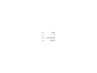
Linear Congruential Generators (LCG) • Let X0 be the seed value (initial value of the sequence). • Then the next values are generated by: • a = the multiplier; c = increment; and m = modulus. • Obviously, Xn can take values: 0, 1, … m-1. • The U(0,1) pseudo-random number is generated by Xn/m. • Values of a, m, and c are chosen such that LCG satisfies the properties of “good” generator.
Linear Congruential Generators (LCG) • For a 32-bit computer, typical values of the parameters are: a = 75 = 16,807 and m = 231 -1. c should be such that the only positive integer that (exactly divides) both c and m is 1. • LCG is bound to “loop.” • Whenever, Xi takes on a value it had previously taken, exactly the same sequence of values is generated and cycle repeats. • The length of the cycle is called period of a generator. • Length of the period can almost be m. • If in fact the period is m, then it is called full period LCG. • If the period is less than m, the cycle length depends on X0.
Testing random number generators Uniformity test • Check whether the values are uniformly distributed between 0 and 1. • As before, we employ a chi-square test statistic to compare the observed frequency and expected frequency of observations in an interval. • We create k intervals and count the number of times the observation falls in a particular interval. If the r.v. generated are U(0,1), the expected frequency should be same for each (equal-sized) interval.
Testing random number generators Serial test • Generalization of the chi-square test in higher dimensions. If individual values are uniformly distributed, then the vector in d-dimensions should be uniformly distributed over a hyper-cube [0,1]d. • Alternately, if individual values are correlated, the distribution of the d-vectors will deviate from d-dimensional uniformity. • Thus, serial test indirectly tests for independence of individual observations.
Testing random number generators Runs test • Directly tests for independence. • We examine the sequence of values for unbroken subsequence of maximal length within which the Ui’s grow monotonically. Such a sequence is called run up.
Testing random number generators • The test statistic is calculated as: where A and b are given matrices. • Turns out that the test statistic R has chi-square distribution. • So this calculated value can be compared with the tabular value to check for the hypothesis of independence.
Generating random variates • Activity of obtaining an observation on (or a realization of) a random variable from desired distribution. • These distributions are specified as a result of activities discussed in last chapter. • Here, we assume that the distributions have been specified; now the question is how to generate random variates with this distributions to run the simulation experiment. • The basic ingredient needed for everymethod of generating random variates from anydistributionis a source of IID U(0,1) random variates. • Hence, it is essential that a statistically reliable U(0,1) random number generator be available.
Requirements from a method Exactness • As far as possible use methods that results in random variates with exactly the desired distribution. • Many approximate techniques are available, which should get second priority. • One may argue that the fitted distributions are approximate anyways, so an approximate generation method should suffice. But still exact methods should be preferred. • Because of huge computational resources, many exact and efficient algorithms exist.
Requirements from a method Efficiency • Efficiency of the algorithm (method) in terms of storage space and execution time. • Execution time has two components: set-up time and marginal execution time. • Set-up time is the time required to do some initial computing to specify constants or tables that depend on the particular distribution and parameters. • Marginal execution time is the incremental time required to generate each random variate. • Since in a simulation experiment, we typically generate thousands of random variates, marginal execution time is far more than the set-up time.
Requirements from a method Complexity • Of the conceptual as well as implementational factors. • One must ask whether the potential gain in efficiency that might be experienced by using a more complicated algorithm is worth the extra effort to understand and implement it. • “Purpose” should be put in context: a more efficient but more complex algorithm might be appropriate for use in permanent software but not for a “one-time” simulation model. Robustness • When an algorithm is efficient for all parameter values.
Inverse transformation method • We wish to generate a random variate X that is continuous and has a distribution function that is continuous and strictly increasing when 0 < F(x) < 1. • Let F-1 denote the inverse of the function F. • Then the inverse transformation algorithm is: • Generate U ~ U(0,1) • Return X = F-1(U). • To show that the returned value X has the desired distribution F, we must show . How?
Inverse transformation method • This method can be used when X is discrete too. Here, where, p(xi) = Pr{X = xi} is the probability mass function. • We assume that X can take only the values x1, x2,… such that x1 < x2 < … • The algorithm then is: • Generate U ~ U(0,1). • Determine the smallest integer I such that , and return X = xI.
Inverse transformation method Advantages: • Intuitively easy to understand. • Helps in variance reduction. • Helps in generating rank order statistics. • Helps in generating random variates from truncated distributions. Disadvantages: • Closed form expression for F-1 may not be readily available for all distributions. • May not be the fastest and the most efficient way of generating random variates.
Composition • Applicable when the desired distribution function can be expressed as a convex combination of several distribution functions. The general composition algorithm is: • Generate a positive random integer J such that: • Return X with distribution function Fj.
Acceptance-Rejection technique • All the previous methods were direct methods – they dealt directly with the desired distribution function. • This method is a bit indirect. • Applicable to continuous as well as discrete case. • We need to specify a function t such that We say that tmajorizes density f. In general, function t will not be a density function, because: • However, the function r(x) = t(x)/c clearly will be a density.
Acceptance-Rejection technique • We should be able to (easily) generate a random variate Y having density r (using one of previous methods). The acceptance-rejection algorithm is: • Generate Y having density r. • Generate U ~ U(0,1) independently of Y. • If Otherwise, go back to Step 1 and try again.
Generating continuous random variates Uniform (a,b) Using inverse-transform method • Generate U ~ U(0,1). • Return X = a + (b-a) U. Exponential (β) Once again, using inverse transform method • Generate U ~ U(0,1). • Return X = - β ln(U).
Generating continuous random variates Normal – N(0,1) • Earliest method from 1958 (still very popular) • Generate U1,U2 as IID U(0,1). • Set • Drawback: If U1 and U2 are generated using adjacent random numbers from LCG, then X1, X2 are not truly independent.
Generating continuous random variates Normal – N(0,1) Polar method • Generate U1,U2 as IID U(0,1). • If W >1, go back to Step 1. Otherwise let
Generating random variates from empirical distribution • For empirical distribution from exact data, recall that: • Algorithm: • Generate U~U(0,1) • Let P = (n-1)U and let • Return:
Generating random variates from empirical distribution For the grouped data. • Generate U ~ U(0,1). • Find the non-negative integer J ( ) such that • Return:
Generating discrete random variates Bernoulli (p) • Generate U ~ U(0,1). • If , return X = 1; otherwise X = 0. Is this a inverse transform method? Binomial (n,p) • Generate Y1, Y2, …, Yn as IID Bernoulli (p) random variates. • Return X = Y1 + Y2 + …+ Yn.
Generating discrete random variates Discrete Uniform (i, j) • Generate U ~ U(0,1). • Return No search is required. We can compute and store ( j-i+1) ahead of time to reduce computation time. This is exactly the inverse transform method, too!
Generating discrete random variates Poisson (λ) • Let a = e- λ, b = 1 and i = 0. • Generate Ui+1 ~ U(0,1) and replace b with bUi+1. If b < a, then X = i. Otherwise go to step 3. • Replace i with i +1 and go back to step 2.

