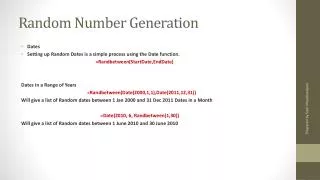
Chapter 7 Random-Number Generation
Chapter 7 Random-Number Generation. Banks, Carson, Nelson & Nicol Discrete-Event System Simulation. Purpose & Overview. Discuss the generation of random numbers. Introduce the subsequent testing for randomness: Frequency test Autocorrelation test. Properties of Random Numbers.

Chapter 7 Random-Number Generation
E N D
Presentation Transcript
Chapter 7 Random-Number Generation Banks, Carson, Nelson & Nicol Discrete-Event System Simulation
Purpose & Overview • Discuss the generation of random numbers. • Introduce the subsequent testing for randomness: • Frequency test • Autocorrelation test.
Properties of Random Numbers • Two important statistical properties: • Uniformity • Independence. • Random Number, Ri, must be independently drawn from a uniform distribution with pdf: Figure: pdf for random numbers
Generation of Pseudo-Random Numbers • “Pseudo”, because generating numbers using a known method removes the potential for true randomness. • Goal: To produce a sequence of numbers in [0,1] that simulates, or imitates, the ideal properties of random numbers (RN). • Important considerations in RN routines: • Fast • Portable to different computers • Have sufficiently long cycle • Replicable • Closely approximate the ideal statistical properties of uniformity and independence.
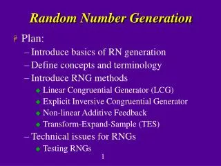
Techniques for Generating Random Numbers • Linear Congruential Method (LCM). • Combined Linear Congruential Generators (CLCG). • Random-Number Streams.
Linear Congruential Method [Techniques] • To produce a sequence of integers, X1, X2, … between 0 and m-1 by following a recursive relationship: • The selection of the values for a, c, m, and X0 drastically affects the statistical properties and the cycle length. • The random integers are being generated [0,m-1], and to convert the integers to random numbers: The modulus The multiplier The increment
Example [LCM] • Use X0 = 27, a = 17, c = 43, and m = 100. • The Xi and Ri values are: X1 = (17*27+43) mod 100 = 502 mod 100 = 2, R1 = 0.02; X2 = (17*2+43) mod 100 = 77, R2 = 0.77; X3 = (17*77+43) mod 100 = 52, R3 = 0.52; …
Characteristics of a Good Generator[LCM] • Maximum Density • Such that he values assumed by Ri, i = 1,2,…, leave no large gaps on [0,1] • Problem: Instead of continuous, each Ri is discrete • Solution: a very large integer for modulus m • Approximation appears to be of little consequence • Maximum Period • To achieve maximum density and avoid cycling. • Achieve by: proper choice of a, c, m, and X0. • Most digital computers use a binary representation of numbers • Speed and efficiency are aided by a modulus, m, to be (or close to) a power of 2.
Combined Linear Congruential Generators[Techniques] • Reason: Longer period generator is needed because of the increasing complexity of stimulated systems. • Approach: Combine two or more multiplicative congruential generators. • Let Xi,1, Xi,2, …,Xi,k, be the ith output from k different multiplicative congruential generators. • The jth generator: • Has prime modulus mj and multiplier aj and period is mj-1 • Produces integers Xi,j is approx ~ Uniform on integers in [1, m-1] • Wi,j = Xi,j -1 is approx ~ Uniform on integers in [1, m-2]
Combined Linear Congruential Generators[Techniques] • Suggested form: • The maximum possible period is: The coefficient: Performs the subtraction Xi,1-1
Combined Linear Congruential Generators[Techniques] • Example: For 32-bit computers, L’Ecuyer [1988] suggests combining k = 2 generators with m1 = 2,147,483,563, a1 = 40,014, m2 = 2,147,483,399 and a2 = 20,692. The algorithm becomes: Step 1: Select seeds • X1,0 in the range [1,2,147,483,562] for the 1st generator • X2,0 in the range [1,2,147,483,398] for the 2nd generator. Step 2: For each individual generator, X1,j+1 = 40,014X1,j mod 2,147,483,563 X2,j+1 = 40,692X1,j mod 2,147,483,399. Step 3: Xj+1 = (X1,j+1 - X2,j+1 ) mod 2,147,483,562. Step 4: Return Step 5: Set j = j+1, go back to step 2. • Combined generator has period: (m1 – 1)(m2 – 1)/2 ~ 2 x 10¹⁸
Random-Numbers Streams[Techniques] • The seed for a linear congruential random-number generator: • Is the integer value X0 that initializes the random-number sequence. • Any value in the sequence can be used to “seed” the generator. • A random-number stream: • Refers to a starting seed taken from the sequence X0, X1, …, XP. • If the streams are b values apart, then stream i could defined by starting seed: • Older generators: b = 105; Newer generators: b = 1037. • A single random-number generator with k streams can act like k distinct virtual random-number generators • To compare two or more alternative systems. • Advantageous to dedicate portions of the pseudo-random number sequence to the same purpose in each of the simulated systems.
Tests for Random Numbers • Two categories: • Testing for uniformity: H0: Ri ~ U[0,1] H1: Ri ~ U[0,1] • Failure to reject the null hypothesis, H0, means that evidence of non-uniformity has not been detected. • Testing for independence: H0: Ri ~ independently H1: Ri ~ independently • Failure to reject the null hypothesis, H0, means that evidence of dependence has not been detected. • Level of significance a, the probability of rejecting H0 when it is true:a = P(reject H0|H0 is true) / /
Tests for Random Numbers • When to use these tests: • If a well-known simulation languages or random-number generators is used, it is probably unnecessary to test • If the generator is not explicitly known or documented, e.g., spreadsheet programs, symbolic/numerical calculators, tests should be applied to many sample numbers. • Types of tests: • Theoretical tests: evaluate the choices of m, a, and c without actually generating any numbers • Empirical tests: applied to actual sequences of numbers produced. The authors’ emphasis.
Frequency Tests[Tests for RN] • Test of uniformity • Two different methods: • Kolmogorov-Smirnov test • Chi-square test
Kolmogorov-Smirnov Test [Frequency Test] • Compares the continuous cdf, F(x), of the uniform distribution with the empirical cdf, SN(x), of the N sample observations. • We know: • If the sample from the RN generator is R1, R2, …, RN, then the empirical cdf, SN(x) is: • Based on the statistic: D = max| F(x) - SN(x)| • Sampling distribution of D is known (a function of N, tabulated in Table A.8.) • A more powerful test, recommended.
Kolmogorov-Smirnov Test [Frequency Test] • Example: Suppose 5 generated numbers are 0.44, 0.81, 0.14, 0.05, 0.93. Arrange R(i) from smallest to largest Step 1: D+ = max {i/N – R(i)} Step 2: D- = max {R(i) - (i-1)/N} Step 3: D = max(D+, D-) = 0.26 Step 4: For a = 0.05, Da = 0.565 > D Hence, H0 is not rejected.
Chi-square test [Frequency Test] • Chi-square test uses the sample statistic: • Approximately the chi-square distribution with n-1 degrees of freedom (where the critical values are tabulated in Table A.6) • For the uniform distribution, Ei, the expected number in the each class is: • Valid only for large samples, e.g. N >= 50 n is the # of classes Ei is the expected # in the ith class Oi is the observed # in the ith class
Tests for Autocorrelation[Tests for RN] • Testing the autocorrelation between every m numbers (m is a.k.a. the lag), starting with the ith number • The autocorrelation rim between numbers: Ri, Ri+m, Ri+2m, Ri+(M+1)m • M is the largest integer such that • Hypothesis: • If the values are uncorrelated: • For large values of M, the distribution of the estimator of rim, denoted is approximately normal.
Tests for Autocorrelation[Tests for RN] • Test statistics is: • Z0 is distributed normally with mean = 0 and variance = 1, and: • If rim > 0, the subsequence has positive autocorrelation • High random numbers tend to be followed by high ones, and vice versa. • If rim < 0, the subsequence has negative autocorrelation • Low random numbers tend to be followed by high ones, and vice versa.
Example [Test for Autocorrelation] • Test whether the 3rd, 8th, 13th, and so on, for the following output on P. 265. • Hence, a = 0.05, i = 3, m = 5, N = 30, and M = 4 • From Table A.3, z0.025 = 1.96. Hence, the hypothesis is not rejected.
Shortcomings [Test for Autocorrelation] • The test is not very sensitive for small values of M, particularly when the numbers being tests are on the low side. • Problem when “fishing” for autocorrelation by performing numerous tests: • If a = 0.05, there is a probability of 0.05 of rejecting a true hypothesis. • If 10 independence sequences are examined, • The probability of finding no significant autocorrelation, by chance alone, is 0.9510 = 0.60. • Hence, the probability of detecting significant autocorrelation when it does not exist = 40%
Summary • In this chapter, we described: • Generation of random numbers • Testing for uniformity and independence • Caution: • Even with generators that have been used for years, some of which still in used, are found to be inadequate. • This chapter provides only the basic • Also, even if generated numbers pass all the tests, some underlying pattern might have gone undetected.