Download

1 / 23
230 likes | 433 Vues
Workshop 7A Diagnostics Tools for Surface Body Contact. Workbench-Mechanical Structural Nonlinearities. Workshop 7A: Diagnostics. Goal Diagnose convergence trouble with surface body contact model Model Description 3D Spring plate – Surface Body 3D Rigid Target Body Linear steel material

E N D
Workshop 7ADiagnostics Tools for Surface Body Contact Workbench-MechanicalStructural Nonlinearities
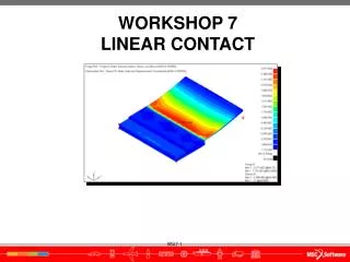
Workshop 7A: Diagnostics • Goal Diagnose convergence trouble with surface body contact model • Model Description • 3D Spring plate –Surface Body • 3D Rigid Target Body • Linear steel material • Meshed with 3D SHELL elements • Spring Fixed support at one end, A • Rigid Body displaced into Spring 19mm
… Workshop 7A: Diagnostics Steps to Follow: • Start an ANSYS Workbench session. Browse for and open “W7a-contact-diagnostics.wbpj” project file.
… Workshop 7A: Diagnostics The project Schematic should look like the picture to the right. • From this Schematic, you can see that the Engineering (material) Data and Geometry have already been defined (green check marks). • It remains to set up and run the FE model in Mechanical • Highlight the Engineering Data Cell and open by clicking on the Right Mouse Button (RMB)=>Edit to verify the linear material properties. • Verify that the units are in Metric(Tonne,mm,..) system. If not, fix this by clicking on… • Utility Menu=>Units=>Metric(Tonne, mm,..)
… Workshop 7A: Diagnostics • Return to Project Schematic • Utility Menu > Return to Project • Double click on the Model Cell to open the FE Model (Mechanical Session) (or RMB=>Edit…)
… Workshop 7A: Diagnostics • Once inside the Mechanical application, verify the working unit system • “Unit > Metric (mm,kg,N,s,mV,mA)” • The spring assembly is already set up with frictionless contact pairs, a fixed boundary condition and a displacement load on the rigid component. • Highlight the entities beneath each folder to become familiar with the model and to confirm that it is properly supported and loaded and ready to solve.
… Workshop 7A: Diagnostics • Confirm the Analysis Settings Specifications as shown: • Run the Solution…
… Workshop 7A: Diagnostics • After solution run is complete, highlight the Solution Information folder and scroll to near the bottom of the output. • Even with the frictionless contact defined and with auto time stepping and large deflection turned On, and plenty of substeps, this solves in one iteration!
… Workshop 7A: Diagnostics • Review the Total Deformation results. • Something is wrong. The contact relationship between the two parts has obviously failed.
… Workshop 7A: Diagnostics With 25 initial substeps and Auto Time Stepping turned On, the contact should have engaged. In an effort to determine the problem, we will evaluate what the initial condition of the contact pairs are. • Highlight the Connections Folder: RMB> Insert> Contact Tool • Highlight the Contact Tool: RMB>Initial Information>Generate Initial Contact Results. This will run a partial solve to establish initial contact parameters (i,e. Initial status, gap, penetration, etc…).
… Workshop 7A: Diagnostics • Review the Initial Contact Information. • Note the following: • The two active pairs both have an initial status of “Far Open” • Both pairs have a pinball radius of 4mm. Is 4mm enough?
… Workshop 7A: Diagnostics • By studying a profile of the undeformed geometry we can see that the initial gap is less then 1.50mm. Hence, the Pinball Radius of 4mm should be sufficient for this contact pair to be in an initial status of ‘near-open’. Rigid Target Spring
… Workshop 7A: Diagnostics • Highlight the contact region representing the contact between the spring and target. • In order for contact to work properly, the contact element normals must be facing the target element normals. • Recall that surface bodies are meshed with shell elements that have a ‘top’ and a ‘bottom’ face. The reason this contact pair is not working is because the contact normals are on the wrong side of the surface body with normals that face away from the target. This needs to be reversed. Target element normal direction Contact element normal direction
… Workshop 7A: Diagnostics • From the details window of the contact region, switch the ‘contact shell face’ from Bottom to Top . The red color highlighting the contact side should switch.
Highlight the Solution Information Branch Set Newton-Raphson Residuals = 3 This will save force imbalance data for the last ‘3’ Newton-Raphson iterations. This is especially helpful information for troubleshooting troubling contact convergence problems. Rerun the solution … Workshop 7A: Diagnostics
… Workshop 7A: Diagnostics • From the Solution Information Branch, the contact is now engaging, but the solution fails to converge after several iterations.
… Workshop 7A: Diagnostics These first two converged substeps likely represent the trivial solutions that occur as the small gap between the two parts is being closed and no contact has been made yet. This first spike in the Newton-Raphson residual (measure of imbalance) likely occurs at the point when contact first engages. From there on out, the solution struggles and fails after two bisections and many iterations to find a balance.
… Workshop 7A: Diagnostics A plot of Newton-Raphson Residual (measure of force imbalance in the model) confirms that the point where contact is engaged is the source of the highest imbalance .
… Workshop 7A: Diagnostics • Highlight both Contact Regions and change the contact specifications in the details window. • Re-run the solution Augmented Lagrange is recommended for general contact Reducing the contact stiffness factor will reduce the calculated force generated at the contact surface and thereby reduce the imbalance
… Workshop 7A: Diagnostics The solution now converges very nicely with no bisections
… Workshop 7A: Diagnostics • Review the Total Deformation results. • Although this solution is now converged, notice the excessive penetration. This is because, by default the shell contact detection points are at the midplane of the shells. • This can be remedied by adding a command object to the contact elements with the following command: KEYOPT,cid,11,1 (refer to Element manual documentation on CONTA174 and the KEYOPT command) • This command will include an adjustment for the shell thickness.
… Workshop 7A: Diagnostics • EXTRA CREDIT !! • Highlight each Contact Region and RMB > Insert > Commands • Inside the command object and type the command as shown • Re-run the solution * * Refer to Element Reference documentation on CONTA174 along with Command Manual documentation on ‘KEYOPT’
… Workshop 7A: Diagnostics • Review the Total Deformation results as before. • Shell thickness is now properly accounted for.


![Contact [TC]² for Perfect Body Measurements](https://cdn4.slideserve.com/8150677/contact-tc-for-perfect-body-measurements-dt.jpg)


![[READ DOWNLOAD] Job's Body: Ahandbook for body workshop](https://cdn7.slideserve.com/12588272/slide1-dt.jpg)