THE MULTINOMIAL DISTRIBUTION AND ELEMENTARY TESTS FOR CATEGORICAL DATA
1.43k likes | 1.72k Vues
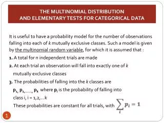
THE MULTINOMIAL DISTRIBUTION AND ELEMENTARY TESTS FOR CATEGORICAL DATA. It is useful to have a probability model for the number of observations falling into each of k mutually exclusive classes. Such a model is given by the multinomial random variable , for which it is assumed that :

THE MULTINOMIAL DISTRIBUTION AND ELEMENTARY TESTS FOR CATEGORICAL DATA
E N D
Presentation Transcript
THE MULTINOMIAL DISTRIBUTION AND ELEMENTARY TESTS FOR CATEGORICAL DATA It is useful to have a probability model for the number of observations falling into each of k mutually exclusive classes. Such a model is given by the multinomial random variable, for which it is assumed that : 1. A total for n independent trials are made 2. At each trial an observation will fall into exactly one of k mutually exclusive classes 3. The probabilities of falling into the k classes are p1, p2,…….,pkwhere piis the probability of falling into class i, i = 1,2,…k These probabilities are constant for all trials, with
If k =2, we have the Binomial distribution. Let us define : X1to be the number of type 1 outcomes in the n trials, X2to be the number of type 2 outcomes, . . Xkto be the number of type k outcomes. As there are n trials,
The joint probability function for these RV can be shown to be : where For k=2, the probability function reduces to which is the Binomial probability of - successes in n trials, each with probability of success .
EXAMPLE A simple example of multinomial trials is the tossing of a die n times. At each trial the outcome is one of the values 1, 2, 3, 4, 5 or 6. Here k=6.If n=10 , the probability of 2 ones, 2 twos, 2 threes, no fours, 2 fives and 2 sixes is : To testing hypotheses concerning the , the null hypothesis for this example, states that the die is fair. vs is false which, of course, means that the die is not fair
The left-hand side can be thought of as the sum of the terms : Which will be used in testing versus where the are hypothesized value of the
In the special case of k=2, there are two-possible outcomes at each trial, which can be called success and failure. A test of is a test of the same null hypothesis ( ). The following are observed an expected values for this situation :
For an α-level test, a rejection region for testing versus is given by We know that Hence, By definition, We have, , and using if and only if
GOODNESS - of – FIT TESTS Thus far all our statistical inferences have involved population parameters like : means, variances and proportions. Now we make inferences about the entire population distribution. A sample is taken, and we want to test a null hypothesis of the general form ; H0 : sample is from a specified distribution The alternative hypothesis is always of the form H1 : sample is not from a specified distribution A test of H0 versus H1is called a goodness-of-fit test. Two tests are used to evaluate goodness of fit : 1. The test, which is based on an approximate statistic. 2. The Kolmogorov – Smirnov (K-S) test. This is called a non parametric test, because it uses a test statistic that makes no assumptions about distribution. The test is best for testing discrete distributions, and the K-S test is best on continuous distributions.
Goodness of Fit ?? A goodness of fit test attempts to determine if a conspicuous discrepancy exists between the observed cell frequencies and those expected under H0 . A useful measure for the overall discrepancy is given by : where O and E symbolize an observed frequency and the corresponding expected frequency. The discrepancy in each cell is measured by the squared difference between the observed and the expected frequencies divided by the expected frequency.
The statistic was originally proposed by Karl Pearson (1857 – 1936) , who found the distribution for large n to be approximately a distribution with degrees of freedom = k-1. Due to this distribution, the statistic is denoted by and is called Pearson’s statistic for goodness of fit . Null hypothesis : H0: pi= pio ; i = 1,2, ….k H1: at least one pi is not equal to its specified value. Test statistic : Rejection Region : distribution with d.f = (k-1)
Chi – square statistic first proposed by Karl Pearson in 1900, begin with the Binomial case. Let X1 ~ BIN (n, p1) where 0 < p1 < 1. According to the CLT : for large n, particularly when np1 ≥ 5 and n(1- p1) ≥ 5. As you know, that Q1 = Z2 ≈ χ2 (1) If we let X2 = n - X1 and p2 = 1 - p1 , Because, Hence,
Pearson the constructed an expression similar to Q1 ; which involves X1 and X2 = n - X1 , that we denote by Qk-1 , involving X1 , X2 , ……., Xk-1 and Xk = n - X1 - X2 - …….- Xk-1 Hence, or
EXAMPLE We observe n = 85 values of a – random variable X that is thought to have a Poisson distribution, obtaining : The sample average is the appropriate estimate of λ = E(X) It is given by The expected frequencies for the first three cells are : npi, i= o,1,2 85 p0 = 85 P(X=0) = 85 (0,449) = 38,2 85 p1 = 85 P(X=1) = 85 (0,360) = 30,6 85 p2 = 85 P(X=2) = 85 (0,144) = 12,2
The expected frequency for the cell { 3, 4, 5 } is : 85 (0,047) = 4,0 ; WHY ??? The computed Q3, with k=4 after combination, no reason to reject H0 H0 : sample is from Poisson distribution vs H1 : sample is not from Poisson distribution
EXERCISE The number X of telephone calls received each minute at a certain switch board in the middle of a working day is thought to have a Poisson distribution. Data were collected, and the results were as follows : Fit a Poisson distribution. Then find the estimated expected value of each cell after combining {4,5,6} to make one cell. Compute Q4 , since k=5, and compare it to Why do we use three degrees of freedom? Do we accept or reject the Poisson distribution?
CONTINGENCY TABLES In many cases, data can be classified into categories on the basis of two criteria. For example, a radio receiver may be classified as having low, average, or high fidelity and as having low, average, or high selectivity; or graduating engineering students may be classified according to their starting salary and their grade-point-average. In a contingency table, the statistical question is whether the rowcriteria and column criteriaare independent. The null and alternative hypotheses are H0 : The row and column criteria are independent H1 : The row and column criteria are associated Consider a contingency table with r rows and c columns. The number of elements in the sample that are observed to fall into row class i and column class j is denoted by
The row sum for the ithrow is And the column sum for jthcolumn is The total number of observations in the entire table is The contingency table for the general case is given ON THE NEXT SLIDESHOW :
There are several probabilities of importance associated with the table. The probability of an element’s being in row class i and column class j in the population is denoted by pij The probability of being in row class i is denoted by pi•, and the probability of being in column class j is denoted by p•j Null and alternative hypotheses regarding the independence of these probabilities would be stated as follows : for all pairs (i , j) versus is false As pij , pi•, p•jare all unknown, it is necessary to estimate these probabilities.
and under the hypothesis of independence, , so would be estimated by The expected number of observations in cell (i,j) is Under the null hypothesis, , the estimate of is The chi-square statistic is computed as
The actual critical region is given by If the computed gets too large, namely, exceeds we reject the hypothesis that the two attributes are independent.
EXAMPLE Ninety graduating male engineers were classified by two attributes : grade-point average (low, average, high) and initial salary (low, high). The following results were obtained.
SOLUTION ; ; ; APA ARTINYA ???
EXERCISES 1.Testof the fidelity and the selectivity of 190 radios produced. The results shown in the following table : Fidelity Low Average High Low Selectivity Average High Use the 0,01 level of significance to test the null hypothesis that fidelity is independent of selectivity.
2. A test of the quality of two or more multinomial distributions can be made by using calculations that are associated with a contingency table. For example, n = 100 light bulbs were taken at random from each of three brands and were graded as A, B, C, or D.
Clearly, we want to test the equality of three multinomial distributions, each with k=4 cells. Since under the probability of falling into a particular grade category is independent of brand, we can test this hypothesis by computing and comparing it with . Use .
ANALYSIS OF VARIANCE The Analysis of Variance ANOVA (AOV) is generalization of the two sample t-test, so that the means of k > 2 populations may be compared ANalysisOf VAriance, first suggested by Sir Ronald Fisher, pioneer of the theory of design of experiments. He is professor of genetics at Cambridge University. The F-test, name in honor of Fisher
The name Analysis of Variance stems from the somewhat surprising fact that a set of computations on several variances is used to test the equality of several means IRONICALLY
The term ANOVA appears to be a misnomer, since the objective is to analyze differences among the group means The ANOVA deals with means, it may appear to be misnamed The terminology of ANOVA can be confusing, this procedure is actually concerned with levels of means ANOVA The ANOVA belies its name in that it is not concerned with analyzing variances but rather with analyzing variation in means
DEFINITION: ANOVA, or one-factor analysis of variance, is a procedure to test the hypothesis that several populations have the same means. ANOVA FUNCTION: Using analysis of variance, we will be able to make inferences about whether our samples are drawn from populations having the same means
INTRODUCTION The Analysis of Variance (ANOVA) is a statistical technique used to compare the locations (specifically, the expectations) of k>2 populations. The study of ANOVA involves the investigation of very complex statistical models, which are interesting both statistically and mathematically. The first is referred to as a one-way classification or a completely randomized design. The second is called a two-way classification or a randomized block design. The basic idea behind the term “ANOVA” is that the total variability of all the observations can be separated into distinct portions, each of which can be assigned a particular source or cause. This decomposition of the variability permits statistical estimation and tests of hypotheses.
Suppose that we are interested in kpopulations, from each of which we sample n observations. The observations are denoted by: Yij , i = 1,2,…k ; j = 1,2,…n where Yijrepresents the jthobservation from population i. A basic null hypothesis to test is : H0 : µ1 = µ2 = … =µk that is , all the populations have the same expectation. The ANOVA method to test this null hypothesis is based on an F statistic.
THE COMPLETELY RANDOMIZED DESIGN WITH EQUAL SAMPLE SIZES First we will consider comparison of the true expectation of k > 2 populations, sometimes referred to as the k– sample problem. For simplicity of presentation, we will assume initially that an equal number of observations are randomly sampled from each population. These observations are denoted by: Y11 , Y12 , …… , Y1n Y21 , Y22 , …… , Y2n . . . Yk1 , Yk2 , …… , Ykn
where Yijrepresents the jthobservation out of the n randomly sampled observations from the ithpopulation. Hence,Y12would be the second observation from the first population. In the completely randomized design, the observations are assumed to : 1. Come from normal populations 2. Come from populations with the same variance 3. Have possibly different expectations, µ1 , µ2 , … , µk These assumptions are expressed mathematically as follows : Yij ~ NOR (µi , σ2) ; i = 1,2,...k (*) j = 1,2,…n This equation is equivalent to………….
Yij = µi + εij , with εij~ NID (0, σ2) Where N represents “normally”, I represents “ independently” and D represents “ distributed”. The 0 means for all pairs of indices i and j, and σ2means that Var ( ) = σ2for all such pairs. The parameters µ1 ,µ2 , … ,µkare the expectations of the k populations, about which inference is to be made. The initial hypotheses to be tested in the completely randomized design are : H0 : µ1 = µ2 = … =µk versus H1 : µi≠ µjfor some pair of indices i ≠ j (**)
The null hypothesis states that all of the k populations have the same expectation. If this is true, then we know from equation (*) that all of the Yijobservations have the same normal distribution and we are observing not n observations from each of k populations, but nk observations, all from the same population. The random variable Yijmay be written as : where, defining, So,
Hence, , with and The hypotheses in equation (**) may be restated as : VS (***) The observation has expectation,
The parameters are differences or deviations from this common part of the individual population expectations . If all of the are equal (say to ), then . In this case all of the deviation are zero, because : Hence, the wall hypothesis in equation (***) means that, , these expectations consist only of the common part . The total variability of the observations : , where , is the means of all of the observations. It can be shown, that :
The notation represents the average of the observations from the ithpopulation; that is The last equation, is represented by : SST = SSA + SSE where SST represents the total sum of squares, SSA represents the sum of squares due to differences among populations or treatments, and SSE represents the sum of squares that is unexplained or said to be “ due to error”. The result of ANOVA, usually reported in an analysis of variance table. ANOVA table……….
ANOVA Table for the Completely Randomized Design with Equal Sample Sizes : For an -level test, a reasonable critical region for the alternative hypotheses in equation (**) is
THE COMPLETELY RANDOMIZED DESIGN WITH UNEQUAL SAMPLE SIZES In many studies in which expectation of k>2 populations are compared, the samples from each population are not ultimately of equal size, even in cases where we attempt to maintain equal sample size. For example, suppose we decide to compare three teaching methods using three classes of students. The teachers of the classes agree to teach use one of the three teaching methods. The plan for the comparison is to give a common examination to all of the students in each class after two months of instruction. Even if the classes are initially of the same size, they may differ after two months because students have dropped out for one reason or another. Thus we need a way to analyze the k-sample problem, when the samples are of unequal sizes.
In the case of UNEQUAL SAMPLE SIZE, the observations are denoted by : . . . where, represents the jthobservation from the ithpopulation. For the ithpopulation there are niobservations. In the case of equal sample sizes, ni = n for i = 1,2,…,k. The model assumptions are the same for the unequal sample size case as for the equal sample size case. The are assumed to : 1. Come from normal populations 2. Come from populations with the same variance 3. Have possibly different expectations, µ1, µ2, …, µk
These assumptions are expressed formally as ; i = 1, 2, …, k j = 1, 2, …, ni or as Yij = µi + εij , with εij~ NID (0, σ2) The first null and alternative hypotheses to test are exactly the same as those in the previous section-namely : H0 : µ1 = µ2 = … =µk versus H1 : µi≠ µlfor some pair of indices i ≠ l The model for the completely randomized design may be presented as : with and εij~ NID (0, σ2) In this case the overall mean, , is given by where is the total number of observations.
Here is a weighted average of the population expectations , where the weights are , the proportion of observations coming from the ithpopulation. The hypotheses, can also be restated as versus for at least one i. The observation Yijhas expectation , If H0is true, then , hence all of the have a common distribution. Thus, , under H0.The total variability of the observations is again partitioned into two portions by or SST = SSA +SSE, here
where As before : represents the average of the observations from the ith population. Nis the total number of observations is the average of all the observations Again, SST represents the total sum of squares. SSA represents the sum of squares due to differences among populations or treatments. SSE represents the sum of squares due to error.
The number of Degrees of Freedom for : TOTAL = TREATMENTS + ERROR (N-1) = (k-1) + (N-k) DEGREE OF FREEDOM
The mean square among treatments and the mean square for error are equal to appropriate sum of squares divided by corresponding dof. That is, It can be shown that MSE is an unbiased estimate of σ2, that is : , similarly ; Under hypothesis, has an F-distribution with (k-1) and (N-k) dof. Finally, we reject the null hypothesis at significance level α if :
ANOVA TABLEfor the Completely Randomized Design with unequal sample sizes • Sometimes, SSA be denoted SSTR • SSE be denoted SSER • SST be denoted SSTO
SUMMARY NOTATION FOR A CRD POPULATIONS (TREATMENTS) INDEPENDENT RANDOM SAMPLES
ANOVA F-TEST FOR A CRDwith k treatments H0 : µ1 = µ2 = … =µk (i.e., there is no difference in the treatment means) versus Ha : At least two of the treatment means differ. Test Statistic : Rejection Region :