Statistical Tests to Analyze the Categorical Data
470 likes | 660 Vues
Statistical Tests to Analyze the Categorical Data. Types of Categorical Data. Types of Analysis for Categorical Data. THE CHI-SQUARE TEST. BACKGROUND AND NEED OF THE TEST Data collected in the field of medicine is often qualitative.

Statistical Tests to Analyze the Categorical Data
E N D
Presentation Transcript
THE CHI-SQUARE TEST BACKGROUND AND NEED OF THE TEST Data collected in the field of medicine is often qualitative. --- For example, the presence or absence of a symptom, classification of pregnancy as ‘high risk’ or ‘non-high risk’, the degree of severity of a disease (mild, moderate, severe)
The measure computed in each instance is a proportion, corresponding to the mean in the case of quantitative data such as height, weight, BMI, serum cholesterol. Comparison between two or more proportions, and the test of significance employed for such purposes is called the “Chi-square test”
KARL PEARSON IN 1889, DEVISED AN INDEX OF DISPERSION OR TEST CRITERIOR DENOTED AS “CHI-SQUARE “. (2).
Introduction • What is the 2 test? • 2 is a non-parametric test of statistical significance for bi variate tabular analysis. • Any appropriately performed test of statistical significance lets you know that degree of confidence you can have in accepting or rejecting a hypothesis.
Introduction • What is the 2 test? • The hypothesis tested with chi square is whether or not two different samples are different enough in some characteristics or aspects of their behavior that we can generalize from our samples that the populations from which our samples are drawn are also different in the behavior or characteristic.
Introduction • What is the 2 test? • The 2 test is used to test a distribution observed in the field against another distribution determined by a null hypothesis. • Being a statistical test, 2 can be expressed as a formula. When written in mathematical notation the formula looks like this:
[ ] S ( o - e) 2 e Chi- Square X 2 = Figure for Each Cell
2 = ∑ ^ total of column in which the cell lies 3. E is the expected frequency (O - E)2 E total of row in which the cell lies reject Ho if 2 > 2.,df where df = (r-1)(c-1) • ^ E = (total of all cells) 1. The summation is over all cells of the contingency table consisting of r rows and c columns 2. O is the observed frequency 4. The degrees of freedom are df = (r-1)(c-1)
When using the chi square test, the researcher needs a clear idea of what is being investigate. • It is customary to define the object of the research by writing an hypothesis. • Chi square is then used to either prove or disprove the hypothesis.
Hypothesis • The hypothesis is the most important part of a research project. It states exactly what the researcher is trying to establish. It must be written in a clear and concise way so that other people can easily understand the aims of the research project.
Chi-square test Purpose To find out whether the association between two categorical variables are statistically significant Null Hypothesis There is no association between two variables
Requirements • Prior to using the chi square test, there are certain requirements that must be met. • The data must be in the form of frequencies counted in each of a set of categories. Percentages cannot be used. • The total number observed must be exceed 20.
Requirements • The expected frequency under the H0 hypothesis in any one fraction must not normally be less than 5. • All the observations must be independent of each other. In other words, one observation must not have an influence upon another observation.
APPLICATION OF CHI-SQUARE TEST • TESTING INDEPENDCNE (or ASSOCATION) • TESTING FOR HOMOGENEITY • TESTING OF GOODNESS-OF-FIT
Chi-square test • Objective : Smoking is a risk factor for MI • Null Hypothesis:Smoking does not cause MI
29 21 O O E E 16 34 O O E E Chi-Square MI Non-MI Smoker Non-Smoker
29 21 O O E E 16 34 O O E E Chi-Square MI Non-MI 50 Smoker 50 Non-smoker 45 55 100
^ E = R2C3 n Classification 1 1 2 3 4 c Classification 2 1 R1 2 R2 3 R3 Estimating the Expected Frequencies r Rr ^ (row total for this cell)•(column total for this cell) n E = C1 C2 C3 C4 Cc
21 O E 16 34 O O E E Chi-Square MI Non-MI 50 29 Smoker 50 X 45 100 O 22.5 = 22.5 E 50 Non-smoker 45 55 100
21 O E 16 34 O O E E Chi-Square Alone Others 50 29 Males O 22.5 27.5 E 50 Females 22.5 27.5 45 55 100
Chi-Square • Degrees of Freedomdf = (r-1) (c-1) = (2-1) (2-1) =1 • Critical Value (Table A.6) = 3.84 • X2 = 6.84 • Calculated value(6.84) is greater than critical (table) value (3.84) at 0.05 level with 1 d.f.f • Hence we reject our Ho and conclude that there is highly statistically significant association between smoking and MI.
df ά = 0.05 ά = 0.01 ά = 0.001 1 3.84 6.64 10.83 2 5.99 9.21 13.82 3 7.82 11.35 16.27 4 9.49 13.28 18.47 5 11.07 15.09 20.52 6 12.59 16.81 22.46 7 14.07 18.48 24.32 8 15.51 20.09 26.13 9 16.92 21.67 27.88 10 18.31 23.21 29.59 Chi square table
Age Gender <30 30-45 >45 Total Male 60 (60) 20 (30) 40 (30) 120 Female 40 (40) 30 (20) 10 (20) 80 Total 100 50 50 200 Chi- square test Find out whether the gender is equally distributed among each age group
Test for Homogeneity (Similarity) To test similarity between frequency distribution or group. It is used in assessing the similarity between non-responders and responders in any survey
X2 = 0.439+ 2.571+ 0.003+ 0.020+ 0.013+ 0.075+ 0.022+ 0.125+ 0.219+ 1.231 = 4.718 • Degrees of Freedomdf = (r-1) (c-1) = (5-1) (2-1) =4 • Critical Value of X2 with 4 d.f.f at 0.05= 9.49 • Calculated value(4.718) is less than critical (table) value (9.49) at 0.05 level with 4 d.f.f • Hence we can not reject our Ho and conclude that the distributions are similar, that is non responders do not differ from responders.
df ά = 0.05 ά = 0.01 ά = 0.001 1 3.84 6.64 10.83 2 5.99 9.21 13.82 3 7.82 11.35 16.27 4 9.49 13.28 18.47 5 11.07 15.09 20.52 6 12.59 16.81 22.46 7 14.07 18.48 24.32 8 15.51 20.09 26.13 9 16.92 21.67 27.88 10 18.31 23.21 29.59 Chi square table
Chi-square test Test statistics 1. 2. 3. 4.
Example The following data relate to suicidal feelings in samples of psychotic and neurotic patients:
Example The following data compare malocclusion of teeth with method of feeding infants.
Fisher’s Exact Test: The method of Yates's correction was useful when manual calculations were done. Now different types of statistical packages are available. Therefore, it is better to use Fisher's exact test rather than Yates's correction as it gives exact result.
What to do when we have a paired samples and both the exposure and outcome variables are qualitative variables (Binary).
Problem • A researcher has done a matched case-control study of endometrial cancer (cases) and exposure to conjugated estrogens (exposed). • In the study cases were individually matched 1:1 to a non-cancer hospital-based control, based on age, race, date of admission, and hospital.
can’t use a chi-squared test - observations are not independent - they’re paired. • we must present the 2 x 2 table differently • each cell should contain a count of the number of pairs with certain criteria, with the columns and rows respectively referring to each of the subjects in the matched pair • the information in the standard 2 x 2 table used for unmatched studies is insufficient because it doesn’t say who is in which pair - ignoring the matching
McNemar’s test Situation: • Two paired binary variables that form a particular type of 2 x 2 table • e.g. matched case-control study or cross-over trial
Formula The odds ratio is: f/g The test is: Compare this to the 2 distribution on 1 df
P <0.001, Odds Ratio = 43/7 = 6.1 p1 - p2 = (55/183) – (19/183) = 0.197 (20%) s.e.(p1 - p2) = 0.036 95% CI: 0.12 to 0.27 (or 12% to 27%)
Degrees of Freedomdf = (r-1) (c-1) = (2-1) (2-1) =1 • Critical Value (Table A.6) = 3.84 • X2 = 25.92 • Calculated value(25.92) is greater than critical (table) value (3.84) at 0.05 level with 1 d.f.f • Hence we reject our Ho and conclude that there is highly statistically significant association between Endometrial cancer and Estrogens.
Stata Output | Controls | Cases | Exposed Unexposed | Total -----------------+------------------------+------------ Exposed | 12 43 | 55 Unexposed | 7 121 | 128 -----------------+------------------------+------------ Total | 19 164 | 183 McNemar's chi2(1) = 25.92 Prob > chi2 = 0.0000 Exact McNemar significance probability = 0.0000 Proportion with factor Cases .3005464 Controls .1038251 [95% Conf. Interval] --------- -------------------- difference .1967213 .1210924 .2723502 ratio 2.894737 1.885462 4.444269 rel. diff. .2195122 .1448549 .2941695 odds ratio 6.142857 2.739772 16.18458 (exact)
In Conclusion ! When both the study variables and outcome variables are categorical (Qualitative): Apply (i) Chi square test (ii) Fisher’s exact test (Small samples) (iii) Mac nemar’s test ( for paired samples)