Fluorescence Spectroscopy

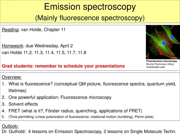
1. Fluorescence Spectroscopy Part I. Background

2. Perrin-Jablonski diagram

3. S is singlet and T is triplet. The S0 state is the ground state and the subscript numbers identify individual states.

4. Energy level of MO n→ p*< p → p*< n→ s*< s → p*< s → s*

5. Singlet & Triplet DS0

6. Characteristics of Excited States • Energy • Lifetime • Quantum Yield • Polarization

7. Stokes shift The Stokes shift is the gap between the maximum of the first absorption band and the maximum of the fluorescence spectrum loss of vibrational energy in the excited state as heat by collision with solvent heat

8. Example: 7-amino-4-methylcoumarin (AMC)

9. Example

10. Example fluorophores fluorescein ethidium bromide bound to DNA.

12. Lifetime

13. Lifetime • Excited states decay exponentially with time • – I = I0e-t/t • I0is the initial intensity at time zero, • Iis the intensity at some later time t • tis the lifetime of the excited state. • kF = 1/ t, where kF is the rate constant for fluorescence.

14. Quantum Yield • Quantum Yield = FF • • FF = number of fluorescence quanta emitted divided by number of quanta absorbed to a singlet excited state • • FF = ratio of photons emitted to photons absorbed • Quantum yield is the ratio of photons emitted to photons absorbed by the system:

15. Quantum Yield

16. Quantum Yield & Structure rigidity

17. Polarization • Molecule of interest is randomly oriented in a rigid matrix (organic solvent at low temperature or room temperature polymer). And plane polarized light is used as the excitation source. • Degree of polarization is defined as P I|| and I^are the intensities of the observed parallel and perpendicular components, ais the angle between thee mission and absorption transition moments. If a is 0° than P = +1/2, and if a is 90° than P = -1/3.

18. Experimental Measurements • Steady-state measurements: F, I • Time-Resolved measurements: t

19. Instruments

20. Inner Filter Effect • At low concentration the emission of light is uniform from the front to the back of sample cuvette. • At high concentration more light is emitted from the front than theback. • Since emitted light only from the middle of the cuvette is detected the concentration must be low to assure accurate FF measurements.

21. Inner Filter Effect

22. Measurement of fluorescence quantum yields em em I0(ex) em em fraction of intensity emitted at that particular wavelength fraction of total fluorescence that is detected If (em)= IAbs (ex).f. f(em).K fluorescence quantum yield absorbed intensity at ex If A0 measured intensity of fluorescence at em If we measure the sample and a standard under the same experimental conditions, keeping ex constant: Standards: Quinine sulfate in H2SO4 1N: f =0.55 Fluorescein in NaOH0.1N: f =0.93 Important : the index of refraction of the two solvents (sample and standard) must be the same

23. Measurement of fluorescence lifetimes pulsed source Start PMT t Time correlated single photon counting: exc. monochromator The TCSPC measurement relies on the concept that the probability distribution for emission of a single photon after an excitation yields the actual intensity against time distribution of all the photons emitted as a result of the excitation. By sampling the single photon emission after a large number of excitation flashes, the experiment constructs this probability distribution. Stop PMT emission monochromator sample different excitation flashes . . . . #events t (nsec)

24. Intrinsic Fluorescence of Proteins and Peptides Lifetime ns Absorption Fluorescence Wavelength nm Absorptivity Wavelength nm Quantum Tryptophan 2.6 280 5,600 348 0.20 Tyrosine 3.6 274 1,400 303 0.14 Phenylalanine 6.4 257 200 282 0.04

27. Tryptophan • Tryptophan, the dominant intrinsic fluorophore, is generally present at about 1mol% in proteins. A protein may possess just one or a few Trp residues, which facilitates interpretation of the spectral data. • Tryptophan is very sensitive to its local environment. It is possible to see changes in emission spectra in response to conformational changes, subunit association, substrate binding, denaturation, and anything that affects the local environment surronding the indole ring. Also, Trp appears to be uniquely sensitive to collisional quenching, either by externally added quenchers, or by nearby groups in the protein. • Tryptophan fluorescence can be selectively excited at 295-305 nm. (to avoid excitation of Tyr)

28. Example:Tyrosine and its derivatives I II III V IV

29. II I III V I IV V III IV II

31. The position and structure of the fluorescence suggests that the indole residue is located in a completely nonpolar region of the protein. These results agree with X-ray studies, which show that the indole group is located in the hydrophobic core of the protein. • In the presence of a denaturing agent, the TrpP emission loses its structure and shifts to 351nm, characteristic of a fully exposed Trp residue. • Changes in emission spectra can be used to follow protein unfolding Emission spectra of Pseudomonas fluorescens azurin Pfl. For 275-nm excitation, a peak is observed due to the tyrosine residue(s)

33. Example Time-resolved protein fluorescence 2=5ns 1=2ns I(,t)=i()exp(-t/i) i Resolution of the contributions of individual tryptophan residues in multi-tryptophan proteins. Fluorescence intensity (A.U.) wavelength (nm) 1=2ns,2= 5ns  em Fluorescence intensity (A.U.) t (ns)

34. Green fluorescent protein (abbreviated GFP Isolated from the Pacific jellyfish Aequorea victoria and now plays central roles in biochemistry and cell biology due to its widespread use as an in vivo reporter of gene expression, cell lineage, protein ­ protein interactions and protein trafficking One of the most important attributes of GFP which makes it so useful in the life sciences is that the luminescent chromophore is formed in vivo, and can thus generate a labeled cellular macromolecule without the difficulties of labeling with exogenous agents.

35. The structure of GFP : eleven-strand beta-barrel wrapped around a central alpha-helix core. This central core contains the chromophore which is spontaneously formed from a chemical reaction involving residues Ser 65, Tyr 66, and Gly 67 (SYG) There is cyclization of the polypeptide backbone between Ser 65 and Gly 67 to form a 5-membered ring, followed by oxidation of Tyr 66. The high quantum yield of GFP fluorescence probably arises from the nearly complete protection of the fluorophore from quenching water or oxygen molecules by burial within the beta-barrel. Ribbon diagram of the Green Fluorescent Protein (GFP) drawn from the wild-type crystal structure. The buried chromophore, which is responsible for GFP's luminescence, is shown in full atomic detail.

36. Wild type GFP from jellyfish has two excitation peaks, a major one at 395 nm and a minor one at 475 nm with extinction coefficient of 30,000 and 7,000 M-1 cm-1, respectively. Its emission peak is at 509 nm in the lower green portion of the visible spectrum. For wild type GFP, exciting the protein at 395 nm leads to rapid quenching of the fluorescence with an increase in the 475 nm excitation band. This photoisomerization effect is prominent with irradiation of GFP by UV light. In a wide range of pH, increasing pH leads to a reduction in fluorescence by 395 nm excitation and an increased sensitivity to 475 nm excitation.

37. Melittin GIGAVLKVLT TGLPALISWI KRKRQQX

38. Example Carboxyfluorescence Biochemical Education 28 (2000) 171~173

39. Example Carboxyfluorescence Quenching Effect

40. Example Carboxyfluorescence pH Effect