Evaluating Parallel Performance: Insights from the ZPL Project
In parallel computing, performance is the ultimate measure of success. This piece discusses findings from the ZPL project, highlighting how the allocation of physical processors affects computational efficiency. The ZPL framework operates under the assumption that many points can be assigned to each processor, influencing local data motion and reducing communication needs during elementwise operations. By analyzing how ZPL performs relative to the CTA Parallel Machine Model, we can derive insights on optimizing performance in machine-independent programming languages.

Evaluating Parallel Performance: Insights from the ZPL Project
E N D
Presentation Transcript
Parallel Performance So far the focus has been on finding good ways to solve problems in a way that underconstrains the specification, and thus permits parallel execution. Now, consider the matter of how much performance is actually achieved. Work reported is from the ZPL project: Brad Chamberlain, Sun-Eun Choi, E Chris Lewis, Calvin Lin, Derrick Weathersby
The Goal In parallel computing, performance is the only measure of success • In ZPL, and in any programming language intended for writing fast programs, the programmer needs to know approximately how the program will run in order to make decisions about alternate solutions • For machine independent languages, this means that only an estimate of performance is possible, but that has proved sufficient in sequential computing
CTA C . . . vN vN vN vN Interconnection Network Recall The CTA Parallel Machine Model • ZPL uses the CTA as its abstract execution engine • Relevant properties emphasize concurrency, locality • P = number of processors • = off processor latency, large • Communication network = unspecified, fixed low degree • “Thin” global communication capability • CTA is implemented by existing parallel machines
P0 a1+b1 Allocating Processors To a Computation To understand how effective our programming is, it is necessary to consider how physical processors will be applied to the computation • For data parallel computations such as those expressible with ZPL’s dense arrays, the one-point-per-processor view, dubbed virtual processor view by Steele and Hillis, is popular • Think of a logical processor performing the task at each point in a parallel operation • 1Pt/Proc is very intuitive P1 P2 P3 P4 P5 a2+b2 a3+b3 a4+b4 a5+b5 a6+b6
ZPL Assumes Many Pts/Proc ZPL allocates arrays to processors so that many contiguous elements are assigned to each processor • The array allocation rules: • Union the regions, compute bounding region • Accept processor number and arrangement from command line • 1D and 2D processor grids are (presently) available • Allocate the bounding region, inducing array allocation • nPt/Proc is just as natural as 1Pt/Proc P0 P1 P2 P3
Implications For Array Allocation The rules imply arrays will have standard distributions • 1D arrays have contiguous range of indices allocated to each processor • 2D arrays are allocated as blocks, panels or strips • 3D and greater? Project to 2D and allocate as 2D arrays
Fundamental Fact of ZPL Allocation The ZPL allocation scheme has the property that for any arrays A, B defined on index i,...,k, elements A[i,...,k], B[i,...,k] are stored on the same processor Corllary: Operations like [R] ... A + B ... do not require any communication Pi [i,...,k]
P0 P0 P1 P2 a1+b1 a2+b2 a3+b3 1Pt/Proc vs nPt/Proc • Obviously, 1Pt/Proc does not represent a realistic situation, but perhaps it is a good metaphor, promoting abundant parallelism • 1Pt/Proc ignores grain size and locality • Forces logical implementation when n > 1 • nPt/Proc accurate for realistic processors • Subsumes 1pt/Proc when n=1 (extreme) • Programmers focus on grain size and locality • Implies standard sequential compiler optimizations It’s hard to throw away parallelism P0 for(i=1;i<=3;i++){ a[i]+b[i]; }
Does It Make Any Real Difference? • Differences between 1Pt/Proc and nPt/Proc are visible for operations like A := B@east • Data motion is required to move B elements • 1Pt/Proc ==> all data sent, no local motion • nPt/Proc ==> some sent, some local motion • Q: How to generalize 1Pt/Proc case? P0 P1 P2 P3 P4 P5 Px b2 b3 b4 b5 b6 b7 b7 a1:=b2 a2:=b3 a3:=b4 a4:=b5 a5:=b6 a6:=b7 P0 P1 b4 b1 b2 b3 b4 b5 b6 b7 a1 a2 a3 a4 a5 a6
Knowing How ZPL Performs • There is a simple rule for how each ZPL operation performs relative to the CTA • Such rules allow one to estimate approximate behavior of ZPL programs in a machine independent way A + B -- Elementwise array operations • No communication • Work comparable to C • Fully parallelizable, WorkC / P Total := 9.0*X^2 + 2.2*X*Y - 3.2*Y^2 + 2 * sqrt(ZZ);
Rules Of Operation II A@east -- @ references including wrap • Nearest neighbor communication with surface/to volume advantage • Local data motion, possibly +<<A -- reduce and scan • Local computation • Ladner/Fischer O(log P) accumulation • Broadcast could be O(log P), but is really less Pi-1 Pi Pi+1
Rules Of Operation III >> [1..n,k] A -- Flood • Multicast defining elements <##[I1,I2] A -- Permutation • (Potential) All-to-all processors communication to distribute routing information implied by I1, I2 • (Potential) All-to-all processors communication to route elements of A Full information is given in Chapter 8 of the ZPL Programmer’s Guide
Analyzing Jacobi Iteration program Jacobi; config var n : integer = 512; eps : float = 0.00001; region R = [1..n, 1..n]; var A, Temp : [R] float; err : float; direction N = [-1, 0]; S = [ 1, 0]; E = [ 0, 1]; W = [ 0,-1]; procedure Jacobi(); [R] begin A := 0.0; [N of R] A := 0.0; [W of R] A := 0.0; [E of R] A := 0.0; [S of R] A := 1.0; repeat Temp := (A@N +A@E +A@W +A@S)/4.0; err := max<< abs(Temp - A); A := Temp; until err < eps; end; end; 0 or negligible performance implications )/4.0; + := ( + +
Analysis repeat Temp := (A@N + A@E + A@W + A@S)/4.0; err := max<< abs(Temp - A); A := Temp; until err < eps; • 4 instances of @-comm + local computation for Temp := (A@N+A@E+A@W+A@S)/4.0 • No communication for abs(Temp - A) • O(log P) per aggregate step and broadcast step for err:=max<< • No communication for A := Temp ... per iteration
WYSIWYG Performance Points to emphasize about the analysis -- • The performance information derives from the CTA and how the compiler maps ZPL programs onto it • Performance is not precise, but given relatively • E.G. reduction is more expensive than flood +<< > >> • To be machine independent, performance could not be given in nanoseconds • Cues indicate when communication is being performed (WYSIWYG): A := A + B; -- No communicaton A := A + B@e; -- Yes, communicaton
CTA C . . . vN vN vN vN Interconnection Network Reconsider Details of @ Communication A@east -- @ references including wrap • Nearest neighbor communication with surface/to volume advantage • Local data motion, possibly Pi-1 Pi Pi+1
@ Comm In The CTA • Charge time for data transmission thru ICN • “Nearest neighbor” not necessarily true • One charge suffices for all transmissions Pi Pi+1
Is This Simplistic Model Accurate? It’s not even close ... but its good enough • Contention in the network makes times vary • On-processor time can dominate network time • Processors may not be adjacent, e.g. fat tree • Processors are not synchronized, so the interval of data transmission could expand • Transmission is not independent of the amount of data transmitted • A better model: + w • Startup time plus for each of w words
Contrary View: Model Accurately “Communication is the most expensive aspect of parallel computing, structure the computation so it optimizes use of communication” • Structuring a program to optimize comm embeds properties of a given computer into the source code • Parallel machines are very different ==> source must be changed for each machine • Wisdom:Do not try to be too accurate. Think of @-Comm as a small, but nonnegligible (fixed) cost, leave optimization to compilers
• • • • • • • • • • • Analyzing The Bounding Box • The bounding box uses four reduces: [R] begin rightedge := max<< X; topedge := max<< Y; leftedge := min<< X; bottomedge := min<< Y; end; • Each reduction has form: • loop to find local max/min • aggregate using LF algorithm • broadcast result to all processors
Compiler Optimizations Notice: Such optimizations result from the compiler’s effectiveness, not directly from the CTA model • Reorder code to • Fuse loops • Combine aggregates • Combine broadcasts loop1 X max aggregate(maxX) broadcast(maxX) loop2 Y max aggregate(maxY) broadcast(maxY) loop3 X min aggregate(minX) broadcast(minX) loop4 Y min aggregate(minY) broadcast(minY) loop X max, Y max, X min, Y min aggregate(maxX, maxY, minX, minY) broadcast(maxX, maxY, minX, minY) • Code runs about 4 times faster
Recall The 8-Connected Components WYSIWYG permits analysis by “inspection” ... Count := 0; repeat Next := Im & (Im@n | Im@nw | Im@w); Next := Next | (Im@w & Im@n & !Im); Conn := Im@e | Im@se | Im@s; Conn := Im & !Next & !Conn; Count += Conn; Im := Next; smore := |<<Next; until !smore; ...
Compiler Basics • An array language gives the illusion of arrays as indivisible objects ... temps/temp removal Next := Next | (Im@w & Im@n & !Im); • Processing arrays creates loops around each statement ... loop fusion/contraction Conn := Im@e | Im@se | Im@s; Conn := Im & !Next & !Conn; Count += Conn; • Communication optimizations ... Next := Im & (Im@n | Im@nw | Im@w); Next := Next | (Im@w & Im@n & !Im); Why is Conn an array? @-comm for Im@n
Annotate According to Rules Local Work, No Comm ... Count := 0; repeat Next := Im & (Im@n | Im@nw | Im@w); Next := Next | (Im@w & Im@n & !Im); Conn := Im@e | Im@se | Im@s; Conn := Im & !Next & !Conn; Count += Conn; Im := Next; smore := |<<Next; until !smore; ... @ Comm required, but only to update boundry. One x-mit at top of loop Log(P) Aggregate and Broadcast What limits the rate of this loop?
Revised Solution Earliest point for computing smore ... Count := 0; repeat Next := Im & (Im@n | Im@nw | Im@w); Next := Next | (Im@w & Im@n & !Im); Conn := Im@e | Im@se | Im@s; smore := |<<Next; Conn := Im & !Next & !Conn; Count += Conn; Im := Next; until !smore; ... loop | Next Aggregate() Broadcast() This optimization makes sense because the CTA assumes asynchronous communication allowing communication to overlap with computation ... Other improvements?
Tale Of Two Multiplies • “It was the best of times” that we wanted from our parallel MM programs, but which of the hall of fame algorithms, Cannon’s or SUMMA, gets the best times? • Analytically, which one is better? • Recall the schema of each program: Cannon’s SUMMA Skew A loop thru n Skew B flood A[,k] loop thru n flood B[k,] C+=A*B C+=A*B rotate A,B Duh?!
Consider The Product Loops What does ZPL’s performance model tell us? Cannon: [Res] C := 0.0; -- Initialize C for k := 1 to n do -- Thru common dim [Res] C := C + A*B ; -- Product & accumulate [right of Lop] wrap A; -- Send first col right [Lop] A := A@right; -- Shift array left [below of Rop] wrap B; -- Send top row down [Rop] B := B@below; -- Shift array up end; SUMMA: [Res] C := 0.0; -- Initialize C [Res] for k := 1 to n do [ ,*] Col := >>[,k] A; -- Flood kth col of A [*, ] Row := >>[k,] B; -- Flood kth row of B C := C+Col*Row;-- Accumulate product end;
Conclusions From Analysis ... • One estimates how a ZPL program performs by using the behavior of the CTA and the WYSIWYG rules of performance • Programming in ZPL is like any language ... it’s possible to write good and bad programs • There is a knack to writing quality ZPL code ... this is in (a small) part due to differences between array and scalar languages, and in (large) part due to the paradigm shift needed for developing parallel algorithms
Preparing For Algorithm Design • Partial reductions aggregate along subarrays, e.g. add rows of array • Dual of flooding ... also requires 2 regions Let var A: [1..n,1..n] float; Colsum: [1..n,1] float; Rowsum: [1,1..n] float; [1..n, 1] Colsum := +<< [1..n,1..n] A; [ 1,1..n] Rowsum := +<< [1..n,1..n] A;
Flooding Is A Powerful Abstraction • Consider the mode of a set of numbers most := 0; count := 0; for i := 1 to n do [i] trial := +<<S; --Select ith elem count := +<<(S = trial); --Occurrences if count > most then --Have a winner? most := count; -- Yes remember it mode := trial; -- And save mode end; end; • Is this a high performance solution? • Embellishment ... • Don’t go to end: for i := 1 to n-count do • What about the reduction? [1..n]
Improvement I Remove the reduction from the loop • Assume positive elements for simplicity ... Count := 0; -- Initialize for i := 1 to n do -- Sweep thru all S Count += S = >>[i]S; -- Record Occurrences end; most := max<< S; -- Figure the best? mode := max<<((most = Count)*S); -- Isolate the mode • Performance ... • n single element broadcasts + local; no early exit • 2 reductions + local [i..n]
Improvement II [1,1..n] Promote the problem to a 2D computation begin ST := <## [Index2,Index1] S; -- Construct Transpose of S Count := +<<[1..n,1..n](>>[1,1..n]S = >>[1..n,1]ST); -- Compare n^2 items, reduce most := max<< S;-- Figure the best? mode := max<<((most = Count)*S); -- Isolate the mode end; • Costs: 1 permute, 2 floods, 1 partial reduction, 2 full reductions, local computation [1..n,1]
Performance of Modes P-Speedup: Time for best sequential solution on 1 proc over time of parallel solution on P processors: Ts/TP 64 2D Flood Solution Speedup 32 16 8 4 Scalar Broadcast Solution 4 8 16 32 64 Processors
A General Idea Problem space promotion (PSP) is a parallel programming technique in which d-dimensional data is processed by solving the problem in a higher dimension d’>d • Flooding (logically) replicates the data • Intermediate data structures need not be built, i.e. PSP is space efficient • Greater parallelism than the control flow solution • Less synchronous solution
Sorting By PSP • Sorting is even easier than mode • Compute the position in the output by counting the number of elements smaller begin ST:= <## [Index2,Index1] S; -- Construct Transpose of S P := +<<[1..n,1..n](>>[1,1..n]S <= >>[1..n,1]ST); -- Compare n^2 items, reduce S := <##[Index1,P] S; -- Reorder input using perm end; • Cost is 2 permutes, 2 floods, partial reduction • Requires n^2 comparisons, though O(n log n) suffices; no early exit [1,1..n] [1..n,1]
Applying PSP to MM ... The idea of flooding for MM generalizes ... region IK = [1..n, 1,1..n]; KJ = [ 1,1..n,1..n]; IJ = [1..n,1..n, 1]; IJK = [1..n,1..n,1..n]; [IK] A2 := <##[Index1,Index3,Index2] A; [KJ] B2 := <##[Index3,Index2,Index1] B; [IJ] C := +<<[IJK] ((>>[IK]A2)*(>>[KJ]B2)); Input B2 A2 C
Matrix Multiplication Performance 3D Flood Solution, No Transp 64 3D Flood Solution SUMMA Speedup 32 16 8 4 4 8 16 32 64 Processors
Recall VQ Compression Loop Code book is input; for each image loop thru CB [R] repeat -- Imput next image, blocked into Im Disto := dist(CB[0],Im);--Init w/dist entry 1 Coding := 0; --Set coding to 1st for i := 1 to 255 do --Sweep thru code bk Distn := dist(CB[i],Im);--dist to ith entry if Disto > Distn then --Is new dist less? Disto := Distn; -- Y, update distance Coding := i; -- record the best end; end; -- Output the compressed image in Coding until no_more_images; No Communication, Except I/O
Very Parallel VQ Solution • region R = [1..n,1..n,0..255]; • var CB = [*,*,0..255]; • ... • -- read in code book, flood into first 2 dimensions • [R] repeat • -- Input blocked image as 1st plane of Im • [1..n,1..n,*] Imrep := >>[,,1] Im; • Temp := dist(CB,Imrep); • Coding := max<<(Index3*(Temp = max<<Temp)); • -- Output the compressed image in Coding • until no_more_images; Why not perform all codebook lookup’s at once? Image CB Imrep
Compiling A Portable/Efficient Language Parallel computers are very different, motivating programmers to use higher level languages • But the compiler must translate the source successfully to each platform with good results • CTA neutralizes much of the complexity • New compiler technology (Factor/Join) promotes many high level optimizations • A critical technology is interprocessor communication -- most compilers use message passing; ZPL uses the Ironman interface
A’ Msg Passing: Lowest Common Denominator Message passing ... • Intended for programmers • Standard libraries (PVM, MPI) give std interface • Most (new) machines have other forms of (more efficient) communication A Pi Pi+1 Strided in memory Scattered in memory Marshalled in pgm Returned to pgm Copied by library Buffered by library Made into Message, “sent” Arrives
Destination location ready Source data is ready A’ Destination data needed Source location to be overwritten Ironman: Compiler Comm Interface • Ironman says what is transferred and when, but not how • Key idea: 4 calls demarcate the legal region of transfer Pi code Pi+1 code A:=1; SR(A); C := ...A’ ... DR(A’); A SV(A); A:=B; DN(A’); D := ... A’...
HW Customize: Binding Ironman Calls With what and when specified by the 4 Ironman calls, the communication is implemented by linking in a library with the specific mechanisms. Pi code Pi+1 code P’gon Msg Pass MPI Asych Msg’s Cray T3E Shmem A:=1; SR(A); C := ...A’ ... DR(A’); Destination Ready Source Ready -- csend MPI_irecv MPI_isend post_ready wait_ready shmem-put post_done SV(A); A:=B; DN(A’); D := ... A’... Destination Needed Source Volatile crecv -- MPI_Wait MPI_Wait wait_done --
Ironman Summary ... • Dumps message passing as compiler communication • Replace w/ 4 calls saying what/when, but not how • DR(), SR(), DN(), SV() • Strategy derives from CTA’s abstract specification • No memory organization stated • Bindings customize to hardware’s mechanism • Versatility covers commercial & prototype machines • message passing (all forms), shmem, shared, differential, ... • Ironman concepts extended to other cases • Collective communication
1000 NAS Multi- Grid SP-2 Targetted Platforms IBM SP-2 Intel Paragon Cray T3D, T3E Clusters SMPs, Workstations, ... SGI Power Challenge, Origin 100 Class “A” Expr HPF (APR) HPF (IBM) HPF (PGI) ZPL Seconds 10 1 1 8 16 32 ZPL In Serious Computations It is easy to analyze small programs,but what about substantial applications? Result: performance with portability Processors
Summary ZPL’s use of CTA permits analysis of programs • The WYSIWYG rules allow the programmer to focus on the expensive communication usage • Programming to achieve good results requires some thinking, but techniques like Problem Space Promotion (PSP) assist • The ZPL compiler performs extensive optimizations and uses the Ironman interface for communication