Download
1 / 37
370 likes | 557 Vues
So, we can now grow long chains, and we are now clever enough to be able to define the associated MICROSTRUCTURE :. Firstly, The ASPECT RATIO can be very counter intuitive: Av. DP ratio L(polyethylene) L(5mm string) 10 10:1 2 nm 5 cm 100 100:1 20 nm 50 cm (shown)

E N D
So, we can now grow long chains, and we are now clever enough to be able to define the associated MICROSTRUCTURE : Firstly, The ASPECT RATIO can be very counter intuitive: Av. DP ratio L(polyethylene) L(5mm string) 10 10:1 2 nm 5 cm 100 100:1 20 nm 50 cm (shown) 1,000 1k:1 200 nm 5 m (short) 10,000 10k:1 2 microns 50 m (usual) 100,000 100k:1 20 microns (a hair) 1/2 km (big)
Most of the REAL macroscopic properties of polymer materials depend on the COIL SIZE, which is related to coil elastic entropy and coil entanglement and knotting. SO, what do the coils look like in an amorphous solid ? or ie: big and springy (left) and highly entangled with the neighbours ? Or compact with little overlap with the neighbours (right) but able to slip and slide easily with each other?
We begin by looking at the THEORY of polymer chain energy and entropy, and specifically how this relates to (predicts) their size and shape: The starting point is the random polymer chain (aka coil) (it doesn’t matter yet what the polymer is)
It can be described as a ‘random walk’ of N steps. After N steps of a random walk, what is your AVERAGE displacement from your starting point? You can expect to find yourself √N steps away from where you started in any direction. RANDOM WALKS show up all over the place in science, as they are the essence of understanding diffusion, kinetics, statistical mechanics, and the SIZES and SHAPES of POLYMER COILS
The usual GAUSSIAN curve of AVERAGE position is where you started, but your displacement after N steps is √N x the step size away. eg: 100 steps: frequency 100 steps left 0 100 steps right
This ( √N x the step size ) average distance applies to random walks around all sorts of parameter space, such as a particle on a 2-d lattice: √N
POLYMER behaviour is mostly ENTROPIC Theory: First Idea: Paul Flory (Stanford): Nobel Prize 1974 Full Theory: Pierre-Gilles de Gennes (Paris): Nobel Prize (in physics) 1991 Some Experiments: NMR: Kurt Wuthrich (Swiss)-Nobel 2002 (½) Mass Spec: Fenn (US), (¼) Tanaka (JP) (¼) 2002
Even though they are all VERY different chemically, polymers can be described very effectively as just: ‘N’ segments of size ‘a’ The total end-to-end length of the chain is therefore a x N, (with ‘a’ usually on the order of a few chemical bonds, 3—10 angstroms). N for random coils can be anywhere from 102—105units a
The prize-winning idea is that the size and shape of polymers can be described as a random walk through space ‘N’ steps of step size ‘a’ = We approximate the coil size the end-to-end random walk distance a√N
A ‘typical’ polymer 1000 units (N = 103) with each a of 3 bonds(5 angstroms), so the total length ≈ (1000 units) x (5 angstroms) = 500 nm= 0.5 μm. ( the width of a human hair is ≈ 30—50 μm, a red blood cell is ~8 μm, and E. Coli about 2 μm ) The size of the random COIL, however, is what is most interesting to us, and we can approximate the coil in ‘vacuum’ as the same in a good solvent and in bulk.
the number of possible conformations of a random polymer coil with N segments (size a) with an end-to-end distance (stretch) of r is : P(r) = 1 / √N e –r2 / 2Na2 P (r) 0 R0 ( = a N 1/2 ) Na
this is for each of 3 dimensions which, after we scale up to macroscopic entropy add up to: ΔS = –3/2 [ r2/R02 + R02/r2 ] r is any radius we want to know about, and R0 is the most likely (highest S) random walk radius a N 1/2 Thus, there is an entropy penalty for stretching the coil (the first term) and for compressing the coil (the second term), from R0 . Does this simple theory really work ?
random walk statistics imply that our 1000 unit polymer chain has a coil size ofr = (5 angstroms) x (1000)1/2 = 160 angstroms 16 nm ( stretched coil was 500 nm ! ) Note: this is a lot of nothing! The coil with the highest entropy, of 16 nm diameter then has a volume of 4/3π r3, = 17,200 nm3
Note: this is a lot of nothing! There are 1000 units in this volume, each with volume 0.125 nm3 (0.5nm x 0.5nm x 0.5nm), so this implies a very low density of <1% PROBLEM: experiments however, show that ‘real’ random coils are usually TWICE this large, over 300 angstroms in diameter. another way of expressing this big difference is to say that the polymer coil size is NOT observed to scale as aN1/2 but as aNx where x (from viscosity and scattering experiments) = 0.6 (not 0.5)
Because it’s an exponent, the difference between x = 0.5 and 0.6 is significant. The problem lies in our original approximation of coil size = diffusion A particle is allowed to cross it’s own path, but a polymer is not. This makes a BIG difference to the statistics !
a computer program can also generate ‘simulated’ polymer coils, of a self-avoiding walk (SAW) : first step 2nd step (random) 2nd step (S.A.W) Units N # configs (rand) ( self-avoiding ) 1 4 4 2 16 12 3 64 36 4 256 100 5 1024 284 6 4096 780 24 2.8 x 10144.6 x 1010
we can understand this big difference between what is observed and our ‘first approach’ by ALSO considering the entropy of the polymer units repelling each other like a diffusing gas this ‘osmotic pressure’ entropy contribution can be estimated simply as the (-) square of the concentration, times the volume. Concentration = N per r3 = N r-3 ( conc )2 = N2r-6
Concentration = N per r3 = N r-3 ( conc )2 = N2r-6 If we multiply this by the volume term a3r3 , then ‘pressure entropy’ = - a3N2r-3 ΔStotal = ΔSpressure + ΔSdeformation = - a3N2r-3 + –3/2 [ r2/R02 + R02/r2 ] = - a3N2r-3 - 3/2 [ r2 R0-2 + R02 r-2 ]
Q: when is this total S function at maximum ? A: when the first derivative dS/dr = 0 : dS/dr = 3 r R0-2 - 3 R02 r-3 – 3 a3N2r-4 if we consider only elongation ( r > R0) then the second term drops out (much smaller than the other 2), and this is equal to zero when : 3 r R0-2 = 3 a3N2r-4
3 r R0-2 = 3 a3N2r-4 or r5 R0-2 = a3N2 or r5 = a3N2 R02 since R0 = aN1/2, R02 = a2N , and r5 = a3N2 a2 N therefore, for highest entropy, r = aN3/5 = aN0.6 We found our mysterious experimental x = 0.6 !
Almost all polymers obey this simple scaling law well, regardless of chemical identity, meaning that the entropy and entanglement are generalizable. even large complex biopolymers can be predicted: wt (g/mol) coil diameter denatured Myoglobin 17,800 ~ 15 nm denatured Hemoglobin 64,450 ~ 32 nm Bovine Serum Albumin 67,500 ~ 33 nm Tobacco Mosaic Virus 39,000,000 ~1500 nm
SO, the a) coil elastic entropy, and b) coil entanglement can be predicted well for most polymers, and only depend on N (= Z = 2DP). The chemical identity of the polymer governs the ‘friction’, the degree of slip, and the slide between neighbouring coils, hence mechanical properties. Unfortunately, predicting the yield point, fracture, or fatigue behaviour of polymers from their structure is still too poor for a perfect theory. It also depends on processing conditions, MW distribution, small amounts of impurities, temperature, rate of deformation, sample history, humidity, phase of the moon…
What we DO KNOW however is that Entropy descriptions work well (describing elasticity and self-assembly), and that there is MUCH different mechanical behaviour above and below the MW limit where neighbouring polymer chains become hopelessly entangled. CRITICAL ENTANGLEMENT LIMITS (text pages 457-460) (viscosity experiments only, but same ideas apply to mechanics) POLYMER Tangle Limit N*POLYMER Tangle Limit N* PMMA 210 P(i-b-ene) 460 PE 275 PVAc 570 P(amide) 324 PS 600 PPO 400 PDMS 630 This depends STRONGLY on the molecular weight distribution, and it is common to add/subtract the low MW component to modify properties.
SO, We now know the macrostructure of polymers, which was derived ‘in vacuum’, and applies well in bulk (the amorphous solid state), effectively the polymer ‘dissolved’ in itself, and also for polymers in solution with ideal solvent Unfortunately, very few solvents are ‘ideal solutions’ for polymers, so a whole new theoretical approach is required to deal with Polymers in Solution. We can begin with a quick review of why anything would want to dissolve in the first place, & when.
ΔGMIX= ΔHMIX — TΔSMIX : This is true for all small molecules and all polymers. The Enthalpy is similar between small and large molecules, but the Entropy is VERY different. The entropy accounts for the fact that for A and B molecules there are many MORE STATES available mixed, than separate enthalpy gain entropy gain
ΔGMIX= ΔHMIX — TΔSMIX : We often forget, but the enthalpy of mixing is almost always POSITIVE (unfavourable), so the driving force is pure ENTROPY. In the absence of secondary interactions, LIKE always prefers LIKE Gibbs energy
This is the essence of ENTROPY: comparing HOW MANY STATES exist for the upper case (very few) and the lower case (very very many) SO, even though there is an enthalpy penalty, most substances will dissolve unless this penalty is very large. The BALANCE between ΔGMIX= ΔHMIX —TΔSMIXpredicts what can dissolve what, and when substances are solids, liquids, and gasses.
ΔGMIX= ΔHMIX — TΔSMIX : So it’s the ENTROPY which drives solvation, and the total number of states available decreases drastically as N increases. SMIX= k ln W Which as N W(molec)/W(polymer) And very large polymers have very little driving force to dissolve. enthalpy gain entropy gain
The ENTHALPY of mixing can be predicted well by considering the attractive forces between the functional groups involved: ΔHMIX /Volume = [ ( ΔE1/V1 )½— ( ΔE2/V2 )½ ] 2 v1v2 Where ΔE1 is the energy of vaporization, V1 is the molar volume of the solvent, and v1 is volume fraction of the solvent. ‘2’ is polymer. The (ΔE/V)½cohesive energy density terms can be expressed as a single ‘solubility’ parameter ‘’ , so ΔHMIX ~ (1—2)2 This solubility parameter is tabulated for most solvents and polymers, so one simply needs to match pairs of for similarity.
This solubility parameter is tabulated for most solvents and polymers, so one simply needs to match pairs of for similarity. Solvent Polymer . Acetone 9.9 p(butadiene) 8.4 Benzene 9.2 p(ethylene) 7.9 Carbon tet 8.6 p(MMA) 9.5 Cyclohex 8.2 p(I-butene) 6.2 Decane 6.6 p(styrene) 9.1 1,4 dioxane 10.0 cellulose triac. 13.6 Methanol 14.5 p(amide 66) 13.6 Toluene 8.9 p(ethylene oxide) 9.9 Water 23.4 p(VinylChloride) 9.6
The ENTROPY of mixing (your book pages 70-75) can be estimated well a) using classical thermodynamics with N2 molecules with mol fraction n2 dissolved in N1 solvent molecules of mol fraction n1: SMIX= -k (N1ln n1 + N2ln n2) Since we are assuming a heat of mixing to be zero for an ideal solution, the Entropy of mixing is always negative, and mixing is spontaneous. b) Using simple statistics of possible arrangements (W) for small molecules of similar size, the total W for arranging N2 solute molecules with N1 solvent molecules on an lattice of No places is: W = No ! / ( N1 ! N2 ! ) Since ln N ! approaches: N ln N – N SMIX= k [(N1+N2)ln (N1+N2 ) - N1ln N1 - N2ln N2]
SMIX= -k (N1ln n1 + N2ln n2) When the solute 2 is a polymer with x chain segments: SMIX= -k (N1ln v1 + N2ln v2) v1 v2 are volume fractions of the solvent and polymer, so are: v1 = N1/ (N1 + xN2) v2 = xN2/ (N1 + xN2) for polymer-polymer solutions: v1 = x1N1/ (x1N1 + x2N2) v2 = x2N2/ (x1N1 + x2N2) Showing that W is reduced considerably when one species is a polymer, and reduced even more considerably when both are. Cases of truly miscible polymers are very rare.
Types of solutions : We had to make some assumptions about heats of mixing when deriving the entropy (IDEAL solutions), and real solutions can be classified: IDEAL solutions have zero heat of mixing (perfect solvent). ATHERMAL solutions have ΔHMIX = 0, but an entropy behaviour more complex than our ΔSMIX equation, and temperature independence. REGULAR solutions have ΔSMIX ~ 0, but ΔHMIX non-zero. IRREGULAR solutions have both ΔSMIX and ΔHMIX deviate from ideal. Deviations are largely due to strong attractive forces between like molecules, and also to volume decrease upon mixing. Correction terms can be used for ΔHMIX which can be zero at a certain temperature.
The ENTHALPY of mixing can be predicted well by considering the attractive forces between the functional groups involved: ΔHMIX /Volume = [ ( ΔE1/V1 )½— ( ΔE2/V2 )½ ] 2 v1v2 The heat of mixing is also widely summarized by one unitless interaction parameter introduced by Flory and Huggins : 1 = ΔHMIX / kTN1v2 Which when combined with our Entropy description provides a GMIX SMIX= -k (N1ln v1 + N2ln v2) GMIX= k T(N1ln v1 + N2ln v2+ 1 N1 v2 ) The difference with being that it describes a polymer-solvent PAIR.
The heat of mixing is also widely summarized by one unitless interaction parameter introduced by Flory and Huggins : 1 = ΔHMIX / kTN1v2 The 1Flory-Huggins parameter for pairs of polymers and solvents is IDEAL when 1= 0.5 (also called the Flory Theta Condition), where properties do not depend on concentration. Often, a Temperature is found for measurements where 1= 0.5 (Theta Temperature). Example: Polystyrene in Cyclohexane at 34 C, 1= 0.500
GMIX= k T(N1ln v1 + N2ln v2+ 1 N1 v2 ) Example: Would you expect Polystyrene of MW 10k g/mol to dissolve in cyclohexane at 34C to a 10% solution by volume? (book p. 75) The number of molecules for v1 = 0.9 and v2 = 0.1: 1) cyclohexane MW = 84 g/mol, density = 0.7785 g/cm3 = 108cm3/mol For v1 = 0.9 then, #mol = 0.0083, and #molec = 5.02 x 1021 = N1 2) polystyrene density = 1.06 g/cm3 = 9400 cm3/mol For v1 = 0.1 then, #mol = 0.0000106, and #molec = 6.38 x 1018 = N2 GMIX= k T(N1ln v1 + N2ln v2+ 1 N1 v2 ) GMIX= -1.24 Jand our polymer just dissolves.
GMIX= k T(N1ln v1 + N2ln v2+ 1 N1 v2 ) GMIX= -1.24 Jand our polymer just dissolves. The coil size is aN0.6 in a good solvent (ideal case) The coil size is aN0.5 in a less good solvent (usual dissolved cases) The coil size is aN0.33 in a bad solvent (collapsed coils)