
Quantifying Uncertainty
E N D
Presentation Transcript
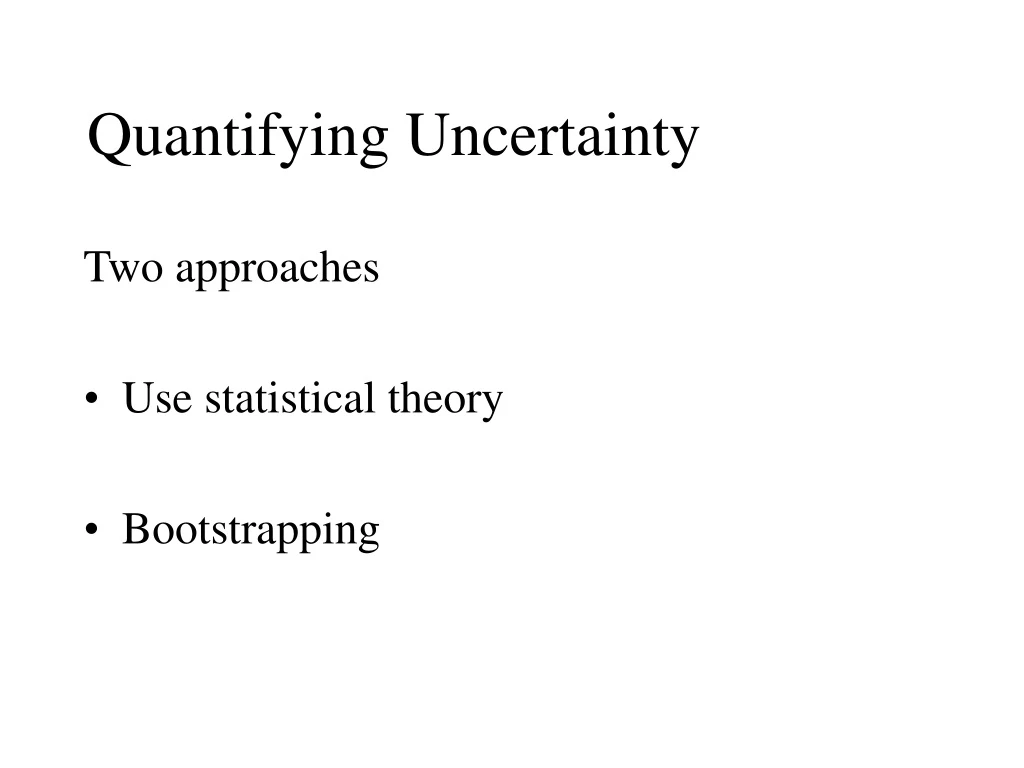
Quantifying Uncertainty Two approaches • Use statistical theory • Bootstrapping
Statistical Theory Uncorrelated Correlated Effective sample size
Significance Statistics • Significance statistics use the standard error: • Confidence Intervals:
Bootstrapping • Motivated by the absence of equations for other accuracy measures (bias, prediction error, confidence intervals) for statistics of interest (correlation, regressions, ACF) • Definition: “The bootstrap is a data-based simulation method for statistical inference.” • Principle: resample with replacement from data. After Efron and Tibshirani, An Introduction to the Bootstrap, 1993
BOOTSTRAP WORLD F * x* = {x*1, x *2, …, x *n} REAL WORLD F x = {x1, x2, …, xn} Empirical Distribution Bootstrap Sample Bootstrap Replication Bootstrapping Unknown Probability Distribution Observed Random Sample Sampling with replacement Statistic of Interest After Efron and Tibshirani, An Introduction to the Bootstrap, 1993
Hillsborough River at Zephyr Hills, September flows Mean = 8621 mgal S = 8194 mgal N = 31 Uncertainty on estimates of the mean One and two standard errors 95% CI and interquartile range from 500 bootstrap samples Millions of gallons
Box-Cox Normality Plot for Monthly September Flows on Alafia R. Using Kolmogorov-Smirnov (KS) Statistic Peak at = -0.39 What is the range of uncertainty on this?
Example for the ks.test • How? • Produce 500 new datasets (x*) of the same length as x by sampling with replacement from x • Find the optimal value for each • Determine the 10th and 90th percentiles to cover 80% of the values calculated.
Look back at the original plot and verify that the original “optimal” value was at the far left of the broad top, which is reflected in this confidence interval. 80% confidence interval 10% 50% 90% -0.425 -0.250 -0.068