3.3 Omitted Variable Bias
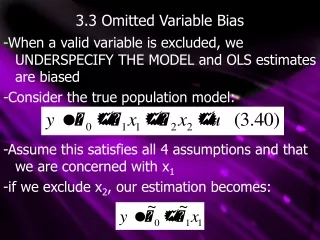
3.3 Omitted Variable Bias. -When a valid variable is excluded, we UNDERSPECIFY THE MODEL and OLS estimates are biased -Consider the true population model:. -Assume this satisfies all 4 assumptions and that we are concerned with x 1 -if we exclude x 2 , our estimation becomes:.

3.3 Omitted Variable Bias
E N D
Presentation Transcript
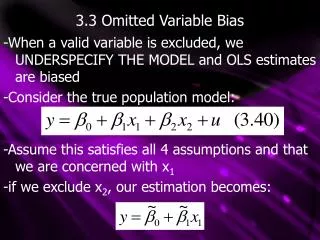
3.3 Omitted Variable Bias -When a valid variable is excluded, we UNDERSPECIFY THE MODEL and OLS estimates are biased -Consider the true population model: -Assume this satisfies all 4 assumptions and that we are concerned with x1 -if we exclude x2, our estimation becomes:
3.3 Omitted Variable Bias -From (3.23) we know that: -where Bhats come from regressing y on ALL x’s and deltatilde comes from regressing x2 on x1 -since deltatilde depends on independent variables, it is considered fixed -we also know from Theorem 3.1 that Bhats are unbiased estimators, therefore:
3.3 Omitted Variable Bias -From this we can calculate Btilde’s bias: -this bias is often called OMITTED VARIABLE BIAS -From this equation, B1tilde is unbiased in two cases: • B2=0; x2 has no impact on y in the true model • deltatilde=0
3.3 Deltatilde=0 -deltatilde is equal to the covariance of x1 and x2 over the variance of x1, all in the sample -deltatilde is equal to zero only if x1 and x2 are uncorrelated -therefore if they are uncorrelated, B1hat is unbiased -it is also unbiased if we can show that:
3.3 Omitted Variable Bias -As B1hat’s bias depends on B2 and deltatilde, the following table summarizes the possible biases:
3.3 Omitted Variable Bias -the SIZE of the bias is also important, as a small bias may not be cause for concern -therefore the SIZE of B2 and deltatilde are important -although B2 is unknown, theory can give us a good idea about its sign -likewise, the direction of correlation between x1 and x2 can be guessed through theory -a positive (negative) bias indicates that given random sampling, on average your estimates will be too large (small)
3.3 Example Take the true regression: Where pasta taste depends on experience making pasta and love -While we can measure years of experience, we can’t measure love, so we find that: What is the bias?
3.3 Example We know that the true B2 should be positive; love improves cooking We can also support a positive correlation between experience and love, if you love someone you spend time cooking for them Therefore B1hat will have a positive bias However, since the correlation between experience and love is small, the bias will likewise be small
3.3 Bias Notes -It is important to realize that the direction of bias is ON AVERAGE -a positive bias on average may underestimate in a given sample If There is an UPWARD BIAS If There is a DOWNWARD BIAS And B1tilde is BIASED TOWARDS ZERO if it is closer to zero than B1
3.3 General Omitted Bias Deriving the direction of omitted variable bias with more independent variables is more difficult -Note that correlation between any explanatory variable and the error causes ALL OLS estimates to be biased. -Consider the true and estimated models: x3 is omitted and correlated with x1 but not x2 Both B1tilde and B2tilde will always be biased unless x1 and x2 are uncorrelated
3.3 General Omitted Bias Since our x values can be pairwise correlated, it is hard to derive the bias for our OLS estimates -If we assume that x1 and x2 are uncorrelated, we can analyze B1tilde’s bias without x2 having an effect, similar to our 2 variable regression: With this formula similar to (3.45), the previous table can be used to determine bias -Note that much uncorrelation is needed to determine bias
3.4 The Variance of OLS Estimators -We now know the expected value, or central tendency, of the OLS estimators -Next we need information on how much spread OLS has in its sampling distribution -To calculate variance, we impose a HOMOSKEDASTICITY (constant error variance) assumption in order to • Simplify variance formulas • Give OLS an important efficiency property
Assumption MLR.5(Homoskedasticity) The error u has the same variance given any values of the explanatory variables. In other words,
Assumption MLR.5 Notes -MLR. 5 assumes that the variance of the error term, u, is the SAME for ANY combination of explanatory variables -If ANY explanatory variable affects the error’s variance, HETEROSKEDASTICITY is present -The above five assumptions are called the GAUSS-MARKOV ASSUMPTIONS -As listed above, they apply only to cross-sectional data with random sampling -time series and panel data analysis require more complicated, related assumptions
Assumption MLR.5 Notes If we let X represent all x variables, combining assumptions 1 through 4 give us: Or as an example: MLR. 5 can be simplified to: Or for example:
3.4 MLR.4 vs. MLR.5 “Assumption MRL. 4 says that the expected value of y, given X, is linear in the parameters – but it certainly depends on x1, x2,….,xk.” “Assumption MLR. 5 says that the variance of y, given X, does not depend on the values of the independent variables.” (bold added)
Theorem 3.2(Sampling Variances of the OLS Slope Estimators) Under assumptions MLR. 1 through MRL. 5, conditional on the sample values of the independent variables, For j= 1, 2,…,k, where Rj2 is the R-squared from regressing xj on all other independent variables (and including an intercept) and SST is the total sample variation in xj:
Theorem 3.2 Notes Note that all FIVE Gauss-Markov assumptions were needed for this theorem Homoskedasticity (MLR. 5) wasn’t needed to prove OLS bias The size of Var(Bjhat) is very important -a large variance leads to larger confidence intervals and less accurate hypothesis tests