Omitted Variable Bias
Omitted Variable Bias. Methods of Economic Investigation Lecture 7. Today’s Lecture. Review Regression Framework Linking last term to this term Understanding conditional expectations Covariates Added and Removed Why is this “Controlling” What if you leave something out?.

Omitted Variable Bias
E N D
Presentation Transcript
Omitted Variable Bias Methods of Economic Investigation Lecture 7
Today’s Lecture • Review Regression Framework • Linking last term to this term • Understanding conditional expectations • Covariates Added and Removed • Why is this “Controlling” • What if you leave something out?
Review: This Course So Far • Do we know what the effect of X is on y? • Defining concepts of “treatment” and “control” • Experimental settings: Explaining the usefulness of Random Assignment • Non-Experimental settings: variation is `as if’ random • In Theory, all you need to do if you have random assignment is take a difference in means • Go backwards a bit…
General Goal in Causal Inference • E(Y| T=1) – E(Y | T=0) or E(Y| T=1, X) – E(Y | T=0, X) • So we need to know how to estimate a conditional expectation function • We’ll worry about if can be causally interpreted later—right now let’s just if we can even show how we could estimate it
What is a conditional expectation • The conditional expectation function (CEF) is the population average of Y with X held fixed • CEF =E[Yi | Xi] • It is a function of X and because X is a random variable, the CEF is itself random • We have been doing the special case where the CEF only takes 2 values • E[Yi | Ti=1] and E[Yi | Ti=0] • In practice, could be continuous but we’ll come back to that
Defining the CEF • For a continuous Y with a density fy(. | X=xi) • Let’s ground this in reality a bit: • The expectation is a concept because we rarely observe the entire population • Generally we’re going to use data to make inferences about the sample CEF • Last term you proved under what conditions and assumptions this sample CEF converges to the population CEF
How is Y related to the CEF • The observed outcome Y can be decomposed into the bit that is explained by X (the CEF) and the unexplained bit ε • Then last term you learned that • CEF is the “best” (in a MMSE sense) summary of the relationship between Y and X • Can also decompose the variance usefully into explained variance and unexplained variance
How is OLS related to this? • If the true CEF is linear, it’s the sample estimate • Example joint normality • Saturated model (different parameter for every possible combination of values for X) • Best Linear Predictor (BLUE) • Best we can relative to other linear estimates • Common justification—local linear approximation • Minimizes Mean Squared Error • Implies it is the best linear approximation to CEF
This should be familiar • You are probably used to thinking OLS as • Turns out that is the thing is the parameter we need to estimate the CEF • And the sample analog that we estimate will converge to the true β (under appropriate conditions
How do we establish Causality? • Conditional Independence Assumption • In words: on average, outcomes would be the same in the treatment and control groups • In Math: Let Y1 be potential outcome if T=1 and Y0 be potential outcome of T=0 • Can write Y = Y0 + (Y1 – Y0)*T • Then CIA: {Y0i,Y1i} independent of Ti(or Ti | Xi) Or E[Yi| T=1 ] – E[Yi| T=0] = E[Y1i – Y0i] • Intuition: since we never observe both Y0 andY1 for any one individual, we want to think on average, the two groups are the same
Selection Bias • The Reason we need CIA: Selection bias • In words: different people choose to be in the treatment or control group. The underlying differences in these people would generate differences in outcomes regardless of the treatment • E(Y| T=1) – E(Y1 | T=0) =E(Y- Y0 |Ti=1) +{E(Y0 | T=1) – E(Y0 | T=0)}
What is generating the bias? • If it’s selection on observables • we can condition on X—estimate the CEF • Convenient that the regression can partial this out: let’s see how • Simple example: 2 variables, T and X, each of which are either zero or one. So, the CEF can have 4 values • E[Y| T=0, X=0]=α • E[Y| T=1, X=0]= α+β • E[Y| T=0, X=1]= α+γ • E[Y| T=1, X=1]= α+β+γ+δ
Extracting β from the estimated CEF • Imagine we estimate each CEF’ • Write a single equation for the CEF E[Y | T, X] = α + βT +γX+δ(T*X) What is β = E[Y| T=1, X=0]- E[Y| T=0, X=0] • Why is X fixed? So we can get β out regression • Generalize this to a continuous X, and we just hold it at some fixed point (e.g. it’s mean) Main effect of T Main effect of X Interaction
What if T didn’t vary with X? • If X has some fixed association with Y independent of T, then the CEF only has 2 values: • E[Y| T=0, X=0]=α • E[Y| T=1, X=0]= α+β • E[Y| T=0, X=1]= α • E[Y| T=1, X=1]= α+β [for ease we can set γ and δ to zero…] • In that case—we’re ok and can exclude X. But we can increase precision because we get 2 estimates of the CEF if we include X
What T and X are correlated? • Then we’ve got a problem • E[Y| T=0, X=0]=α • E[Y| T=1, X=0]= α+β • E[Y| T=0, X=1]= α+γ • E[Y| T=1, X=1]= α+β+γ+δ • If we don’t have X: E[Y | T=1] has two potential values and we cannot say: E[Y | T=1] –E[Y | T=0 ≠ E[Y1 - Y0 | T=1] • Another way to say this is we’ve got “selection on unobservables”
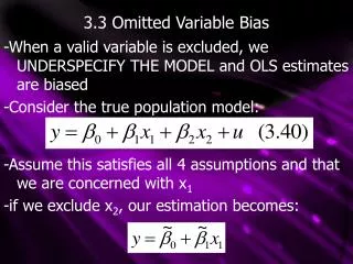
Omitted Variable Bias Formula • Simply from before, suppose δ=0 so our true CEF is: E[Y | T, X] = α + βT +γX (REMEMBER: This means Y = E[Y | T, X] +e) • We estimate
What is happening when we estimate? • What this is doing is given observed Y’s for the various values of T it is choosing the α and β that minimize the mean square error • intuitively, the bias happens because the values of Y’s are changing not only with respect to T but also the unobserved X • In more formal terms we get: Should look familiar True β (this is what we want) Relationship between X and Y
What is relationship between X and T • Pretend we could observe X…then w could think about estimating • Well, we know, since this is OLS and assuming no OVB in this equation that • So our omitted variable bias formula can be re-written as:
Signing your bias • Generally, the concern with OVB is that it biases your estimate upwards. • The sign of the bias will be as follows:
What did we learn today • Conditional Expectation Functions (CEFs) are how we determine “causal effects” • Regressions allow the “best” way to estimate these CEFs • Selection on observables is not something that will bias our estimates • Selection on unobservables is a problem
Next Class • Review of OVB • Error Correction Models • Fixed Effects • Random Effects (interaction terms)