Download
1 / 13
130 likes | 234 Vues
This study explores the generation and destruction of turbulent kinetic energy in various weather scenarios during T-REX, combining aerosol lidar and tower data. Analysis includes Richardson number, turbulence situations, and estimation methods like the Inertial Dissipation Method. Data analysis involves tower locations, wind speed components, Richardson number time series, dissipation rate, and mechanical term distribution. Findings indicate balance and independence in turbulence data, suggesting further investigation across stability conditions and wind environments.

E N D
Spatial and Temporal Features of Mountain Wave Related Turbulence *Željko Večenaj, #Stephan de Wekker & +Vanda Grubišić *Department of Geophysics, Faculty of Science, University of Zagreb, Croatia #Department of Environmental Sciences, University of Virginia, Virginia +Division of Atmospheric Sciences, Desert Research Institute, Reno, Nevada Email: zvecenaj@gfz.hr .
CONTENT • INTRODUCTION • DATA ANALYSIS • RESULTS • CONCLUSIONS
I. INTRODUCTION • OBJECTIVE: • To study the horizontal and vertical structure of TKE generation and destruction in a variety of weather situations during T-REX • To combine aerosol lidar data and towers data • TURBULENT KINETIC ENERGY BALANCE EQUATION:
Richardson number • We are interested in following situations: Ri >> 0 ……… Stable situation Ri << 0 ………. Convectively produced turbulence Ri ≈ 0 ………... Turbulence produced by wind stress
I.1. ESTIMATION OF ε • For evaluation of ε, the Inertial Dissipation Method (IDM) provided by the Kolmogorov’s 1941 hypotheses can be employed • Condition: Taylor’s Hypotheses (TH) of frozen turbulence must be valid (transformation from time to space domain) • Criterion:(e.g. Stull, 1988) M.........Mean horizontal wind speed σM........Standard deviation
Power spectrum density in inertial subrange: (1) • Using TH, ε can be evaluated from (Champagne et al., 1977): (2) ..........mean streamwise velocity component Su(f) ......power spectrum density ..........Kolmogorov’s constant
II. DATA ANALYSIS Figure 1. The map of the area of interest along with the towers locations.
Height of towers: 35 m • 6 vertical levels: 5, 10, 15, 20, 25 and 30 m • CSAT3 ultrasonic anemometers • Sampling rate: 60 Hz • The data are averaged down to 10 Hz for further analysis • period of interest: 02 March 00 UTC to 04 March 00 UTC (IOP1) • Ggccc
Figure 2. East (first row) and north (second row) 10 Hz wind speed components of the observed 6 hr episode (black curve). White curve is the 5 min moving average. Vertical dashed lines denote a period of interest.
Figure 3.The time series of the Bulk Richardson number in the layer between 5 & 30 m (for the west tower between 5 & 25 m).
III. RESULTS Figure 4. Time series of 1 minute dissipation rate values Figure 5. Time series of 15 minute dissipation rate values
Figure 6. Vertical distribu- tion of 15 minutes averages of the 1 min TKE dissipation rate in time for all three towers. Figure 7. Vertical distribu- tion of 15 minutes averages ofthe 1 min mechanical term in time for all three towers.
IV. CONCLUSIONS • We have started to analyze turbulence data from the three NCAR towers • Independence of the averaging period is present • Balance of the mechanical term and the TKE dissipation rate is present • Next steps: (1) To extend this work to the other two towers and to other IOPs/EOPs to investigate spatial and temporal structure in a variety of stability and wind conditions (2) Comparison with estimates/observations from other instruments (wind profiler/lidar/aircraft) Acknowledgments: we would like to thank Steve Oncley for providing turbulence data