Download
1 / 81
930 likes | 1.72k Vues
Energy or Energy Head. Elevation head Velocity head Total head. Energy Head -Elevation Head -Velocity Head -Total Head Momentum Open Channel. Energy or Energy Head. The total energy of water moving through a channel is expressed in total head in feet of water.

E N D
Energy or Energy Head • Elevation head • Velocity head • Total head Energy Head -Elevation Head -Velocity Head -Total Head Momentum Open Channel
Energy or Energy Head • The total energy of water moving through a channel is expressed in total head in feet of water. • This is simply the sum of the the elevation above a datum (elevation head), the pressure head and the velocity head. • The elevation head is the vertical distance from a datum to a point in the stream. • The velocity head is expressed by: Energy Head -Elevation Head -Velocity Head -Total Head Momentum Open Channel
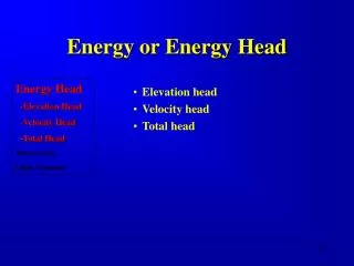
Energy Head Graphical depiction of elevation head, velocity head, and total head. Total head is the sum of velocity head, depth and elevation head. Energy Head -Elevation Head -Velocity Head -Total Head Momentum Open Channel Energy Grade Line headloss Hydraulic Grade Line Veloctiy head (water surface) Depth1 Channel Bottom Elevation Head Depth2 Datum
Momentum Equation Energy Head Momentum -Equation -Forces Open Channel Hydrostatic Forces Friction Forces Weight External Forces
H P=gH Hydrostatic Forces • Hydrostatic Forcesare the forces placed on a control volume by the surrounding water. • The strength of the force is based on depth and can be seen in the following relationship: Energy Head Momentum -Equation -Forces Open Channel Hydrostatic Forces Control Volume Hydrostatic Forces Friction Forces Weight External Forces
Friction Forces Energy Head Momentum -Equation -Forces Open Channel Thefriction forceon a control volume is due to the water passing the channel bottom and depends on the roughness of the channel. Control Volume Friction Force Hydrostatic Forces Friction Forces Weight External Forces
Weight Energy Head Momentum -Equation -Forces Open Channel Theweightof a control volume is due to the gravitational pull on the its mass. Weight = mg Control Volume Weight Hydrostatic Forces Friction Forces Weight External Forces
Streamflow direction Fd Top View of Control Volume External Forces Energy Head Momentum -Equation -Forces Open Channel External Forces (Fd) the forces created by a control volume striking a stationary object. External Forces can be explained by the following equation: Fd=1/2CdrAv2 Hydrostatic Forces Friction Forces Weight External Forces
Steady vs. Unsteady Flow • Fluid properties including velocity, pressure, temperature, density, and viscosity vary in time and space. • A fluid it termed steady if the depth of flow does not change or can be assumed constant during a specific time interval. • Flow is considered unsteady if the depth changes with time. Energy Head Momentum Open Channel -Steady -vs- Unsteady -Uniform -vs- Nonuniform -Supercitical -vs- subcritical -Equations
Uniform and Nonuniform Flow • Uniform Flow is an equilibrium flow such that the slope of the total energy equals the bottom slope. • Nonuniform Flow is a flow of water through a channel that gradually changes with distance. Energy Head Momentum Open Channel -Steady -vs- Unsteady -Uniform -vs- Nonuniform -Supercitical -vs- subcritical -Equations
Super -vs.- Sub Critical Energy Head Momentum Open Channel -Steady-vs.-Unsteady -Uniform-vs. Nonuniform -Sub/Supercritical -Equations
Critical flow: a demonstration Energy Head Momentum Open Channel -Steady-vs.-Unsteady -Uniform-vs. Nonuniform -Sub/Supercritical -Equations If a stone is dropped into a body of water, with no velocity, the waves formed by the water are fairly circular. This is similar to sub-critical flow. No velocity
Critical flow: a demonstration Energy Head Momentum Open Channel -Steady-vs.-Unsteady -Uniform-vs. Nonuniform -Sub/Supercritical -Equations Now, if a velocity is added to the body of water, the waves become unsymmetrical, increasing to the downstream side. This happens as the velocity approaches critical flow. Notice that the wave still moves upstream, though slower than the downstream wave. Small velocity
Critical flow: a demonstration Energy Head Momentum Open Channel -Steady-vs.-Unsteady -Uniform-vs. Nonuniform -Sub/Supercritical -Equations Now if a large velocity is added to the body of water, the wave patterns only go in one direction. This represents the point when flow has gone beyond critical, into the supercritical region. Large velocity
Froude number Energy Head Momentum Open Channel -Steady-vs.-Unsteady -Uniform-vs. Nonuniform -Sub/Supercritical -Froude number -Equations TheFroude numberis a numerical value that describes the type of flow present (critical, supercritical, subcritical), and is represented by the following equation for a rectangular channel: NF = Froude number v = mean velocity of flow g = acceleration of gravity dm = mean (hydraulic) depth
Froude number Energy Head Momentum Open Channel -Steady-vs.-Unsteady -Uniform-vs. Nonuniform -Sub/Supercritical -Froude number -Equations Thegeneralized formula for theFroude numberis as follows: Fr = Froude number Q = Flow rate in the channel B = Top width of water surface A = Area of the channel
B=width of the free water surface A=cross-sectional area of the channel Froude number - mean depth Energy Head Momentum Open Channel -Steady-vs.-Unsteady -Uniform-vs. Nonuniform -Sub/Supercritical -Froude number -Equations • Mean depth is a ratio of the width of the free water surface to the cross-sectional area of the channel.
Froude number Energy Head Momentum Open Channel -Steady-vs.-Unsteady -Uniform-vs. Nonuniform -Sub/Supercritical -Froude number -Equations • TheFroude number can then be used to quantify the type of flow. • If the Froude number isless than 1.0, the flow issubcritical. The flow would would be characterized as tranquil. • If the Froude number isequal to 1.0, the flow iscritical. • If the Froude number isgreater than 1.0, the flow issupercriticaland would be characterized as rapid flowing. This type of flow has a high velocity which can be potentially damaging.
Super-vs.-Subcritical Energy Head Momentum Open Channel -Steady-vs.-Unsteady -Uniform-vs. Nonuniform -Sub/Supercritical -Equations • Critical depth can also be determined by constructing a Specific Energy Curve. • Thecritical depthis the point on the curve with thelowest specific energy. • Any depth greater than critical depth is subcritical flow and any depth less than is supercritical flow.
Subcritical depth Critical depth Supercritical depth Super-vs.-Subcritical
Open Channel Equations • Energy Head • Momentum • Open Channel • -Steady -vs- Unsteady • -Uniform -vs- Nonuniform • -Supercitical -vs- subcritical • -Equations: • Chezy • Manning • Bernoulli • St. Venant • Chezy Equation • Manning’s Equation • Bernoulli Equation • St. Venant Equations
Chezy Equation Energy Head Momentum Open Channel -Chezy Equation -Manning’s -Bernoulli -St. Venant • In 1769, the French engineer Antoine Chezy developed the first uniform-flow formula. • The formula was derived based on two assumptions. First, Chezy assumed that the force resisting the flow per unit area of the stream bed is proportional to the square of the velocity (KV2), with K being a proportionality constant.
Chezy Equation Energy Head Momentum Open Channel -Chezy Equation -Manning’s -Bernoulli -St. Venant • The second assumption was that the channel was undergoing uniform flow. • The difficulty with this formula is determining the value of C, which is the Chezy resistance factor. There are three different formulas for determining C, the G.K. Formula, the Bazin Formula, and the Powell Formula.
Chezy Equation Energy Head Momentum Open Channel -Chezy Equation -Manning’s -Bernoulli -St. Venant • Later on, when Manning's equation was developed in 1889, a relationship between Manning’s “n” and Chezy’s “C” was established. • Finally in 1933, the Manning equation was suggested for international use rather than Chezy’s Equation.
Manning’s Equation Energy Head Momentum Open Channel -Chezy Equation -Manning’s -Bernoulli -St. Venant • In 1889 Robert Manning, an Irish engineer, presented the following formula to solve open channel flow. V = mean velocity in fps R = hydraulic radius in feet S = the slope of the energy line n = coefficient of roughness The hydraulic radius (R) is a ratio of the water area to the wetted perimeter.
Manning’s Equation Energy Head Momentum Open Channel -Chezy Equation -Manning’s -Bernoulli -St. Venant • This formula was later adapted to obtain a flow measurement. This is done by multiplying both sides by the area. • Manning’s equation is the most widely used of all uniform-flow formulas for open channel flow, because of its simplicity and satisfactory results it produces in real-world applications.
Manning’s Equation Energy Head Momentum Open Channel -Chezy Equation -Manning’s -Bernoulli -St. Venant • Note that the equation expressed in the previous slide was the English version of Manning’s equation. • There is also a metric version of Manning’s equation, which replaces the 1.49 with 1. This is done because of unit conversions. • The metric equation is:
Bernoulli Equation Energy Head Momentum Open Channel -Chezy Equation -Manning’s -Bernoulli -St. Venant • The Bernoulli equation is developed from the following equation: This equation states that the elevation (z) plus the depth (y) plus the velocity head (V12/2g) is a constant. The difference being the headlosses - hL
Bernoulli Equation • This equation was then adapted by making a few assumptions. • First, the head loss due to friction is equal to zero. This means the channel is perfectly frictionless surface. • Second, that alpha1 is equal to alpha2 which is equal to 1. The alpha’s are in the original equation to account for a non-uniform velocity distribution. In this case we will assume a uniform distribution which produces the following equation: Energy Head Momentum Open Channel -Chezy Equation -Manning’s -Bernoulli -St. Venant
Bernoulli Equation Energy Head Momentum Open Channel -Chezy Equation -Manning’s -Bernoulli -St. Venant A simplified version of the formula is given below:
Bernoulli Equation Energy Head Momentum Open Channel -Chezy Equation -Manning’s -Bernoulli -St. Venant • Some comments on the Bernoulli equation • Energy only • Headloss in terms of energy • Cannot calculate forces • Limited Effect in “rapidly varying flow”
St. Venant Equations Energy Head Momentum Open Channel -Chezy Equation -Manning’s -Bernoulli -St. Venant The two equations used in modeling are the continuity equation and the momentum equation. Continuity equation Momentum Equation
St. Venant Equations The Momentum Equation can often be simplified based on the conditions of the model. Energy Head Momentum Open Channel -Chezy Equation -Manning’s -Bernoulli -St. Venant Unsteady -Nonuniform Steady - Nonuniform Diffusion or noninertial Kinematic
Simulating the Hydrologic Response Model Types Precipitation Losses Modeling Losses Model Components
Model Types Model Types Precipitation Losses Modeling Losses Model Components • Empirical • Lumped • Distributed
Precipitation Model Types Precipitation -Thiessen -Isohyetal -Nexrad Losses Modeling Losses Model Components • … magnitude, intensity, location, patterns, and future estimates of the precipitation. • … In lumped models, the precipitation is input in the form of average values over the basin. These average values are often referred to as mean aerial precipitation (MAP) values. • … MAP's are estimated either from 1) precipitation gage data or 2) NEXRAD precipitation fields.
Precipitation (cont.) Model Types Precipitation -Thiessen -Isohyetal -Nexrad Losses Modeling Losses Model Components • … If precipitation gage data is used, then the MAP's are usually calculated by a weighting scheme. • … a gage (or set of gages) has influence over an area and the amount of rain having been recorded at a particular gage (or set of gages) is assigned to an area. • … Thiessen method and the isohyetal method are two of the more popular methods.
Thiessen Model Types Precipitation -Thiessen -Isohyetal -Nexrad Losses Modeling Losses Model Components • Thiessen methodis a method for areally weighting rainfall through graphical means.
Isohyetal Model Types Precipitation -Thiessen -Isohyetal -Nexrad Losses Modeling Losses Model Components • Isohyetal methodis a method for areally weighting rainfall using contours of equal rainfall (isohyets).
NEXRAD Model Types Precipitation -Thiessen -Isohyetal -Nexrad Losses Modeling Losses Model Components • Nexradis a method of areally weighting rainfall using satellite imaging of the intensity of the rain during a storm.
Losses Model Types Precipitation Losses Modeling Losses Model Components • … modeled in order to account for the destiny of the precipitation that falls and the potential of the precipitation to affect the hydrograph. • … losses include interception, evapotranspiration, depression storage, and infiltration. • … Interception is that precipitation that is caught by the vegetative canopy and does not reach the ground for eventual infiltration or runoff. • … Evapotranspiration is a combination of evaporation and transpiration and was previously discussed. • … Depression storage is that precipitation that reaches the ground, yet, as the name suggests, is stored in small surface depressions and is generally satisfied during the early portion of a storm event.
Modeling Losses Model Types Precipitation Losses Modeling Losses -SAC-SMA Model Components • … simplistic methods such as a constant loss method may be used. • … A constant loss approach assumes that the soil can constantly infiltrate the same amount of precipitation throughout the storm event. The obvious weaknesses are the neglecting of spatial variability, temporal variability, and recovery potential. • Other methods include exponential decays (the infiltration rate decays exponentially), empirical methods, and physically based methods. • … There are also combinations of these methods. For example, empirical coefficients may be combined with a more physically based equation. (SAC-SMA for example)
Simulating Watershed ResponseInfiltration Long Term –vs.- ShortInfiltration Evapotranspiration Unit Hydrograph Timing Routing Infiltration or “losses” - this section describes the action of the precipitation infiltrating into the ground. It also covers the concept of initial abstraction, as it is generally considered necessary to satisfy the initial abstraction before the infiltration process begins.
Simulating Watershed ResponseInfiltration Long Term –vs.- ShortInfiltration Evapotranspiration Unit Hydrograph Timing Routing Initial Abstraction - It is generally assumed that the initial abstractions must be satisfied before any direct storm runoff may begin. The initial abstraction is often thought of as a lumped sum (depth). Viessman (1968) found that 0.1 inches was reasonable for small urban watersheds. Would forested & rural watersheds be more or less?
Simulating Watershed ResponseInfiltration Long Term –vs.- ShortInfiltration Evapotranspiration Unit Hydrograph Timing Routing Forested & rural watersheds would probably have a higher initial abstraction. The Soil Conservation Service (SCS) now the NRCS uses a percentage of the ultimate infiltration holding capacity of the soil - i.e. 20% of the maximum soil retention capacity.
Simulating Watershed ResponseInfiltration Long Term –vs.- ShortInfiltration Evapotranspiration Unit Hydrograph Timing Routing Infiltration is a natural process that we attempt to mimic using mathematical processes. Some of the mathematical process or simulation methods are conceptual while others are more physically based.
Simulating Watershed ResponseInfiltration Constant Infiltration Rate : A constant infiltration rate is the most simple of the methods. It is often referred to as a phi-index or f-index. In some modeling situations it is used in a conservative mode. The saturated soil conductivity may be used for the infiltration rate. The obvious weakness is the inability to model changes in infiltration rate. The phi-index may also be estimated from individual storm events by looking at the runoff hydrograph. Long Term –vs.- ShortInfiltration Evapotranspiration Unit Hydrograph Timing Routing
Simulating Watershed ResponseInfiltration Long Term –vs.- ShortInfiltration Evapotranspiration Unit Hydrograph Timing Routing Constant Percentage Method : Another very simplistic approach - this method assumes that the watershed is capable of infiltrating or “using” a value that is proportional to rainfall intensity. The constant percentage rate can be “calibrated” for a basin by again considering several storms and calculating the percentage by :
Constant Percentage Example Long Term –vs.- ShortInfiltration Evapotranspiration Unit Hydrograph Timing Routing 2 77.5% infiltrates 1 0
Simulating Watershed ResponseInfiltration Long Term –vs.- ShortInfiltration Evapotranspiration Unit Hydrograph Timing Routing Exponential Decay: This is purely a mathematical function - of the following form: