Boosting for prediction and inference
560 likes | 721 Vues
Boosting for prediction and inference. By Marc Sobel. Sometimes you just need a boost!!!. Learning.

Boosting for prediction and inference
E N D
Presentation Transcript
Boosting for prediction and inference By Marc Sobel
Learning • Consider a setting in which we have training (or labeled) data and test (or unlabeled) data. (Example: (i) learning who are the consumers of a particular product using a training data set in which the consumers are identified.) We would like to ‘learn’ the unlabelled data using the labeled data.
Greedy Algorithms • Greedy algorithms for learning optimize some loss function at each stage. • A) CART (classification and regression trees) • B) MARS (multivariate adaptive regression splines) • C) stepwise regression.
Stepwise regression (from wikipedia) • In this example from engineering, necessity and sufficiency are usually determined by F-tests. For additional consideration, when planning an experiment, computer simulation, or scientific survey to collect data for this model, one must keep in mind the number of parameters, P, to estimate and adjust the sample size accordingly. For K variables, P = 1(Start)+ K(Stage I)+ (K2-K)/2(Stage II)+ 3K(Stage III)= .5K2+ 3.5K + 1. For K<17, an efficientdesign of experiments exists for this type of model, a Box-Behnken design,[4] augmented with positive and negative axial points of length min(2,sqrt(int(1.5+K/4))), plus point(s) at the origin. There are more efficient designs, requiring fewer runs, even for K>16.
MARS (from wikipedia) [use Bayesian Mars – see A.F.M. Smith] • Multivariate adaptive regression splines is a non-parametric technique that builds flexible models by fitting piecewise linear regressions. • An important concept associated with regression splines is that of a knot. Knot is where one local regression model gives way to another and thus is the point of intersection between two splines. • In multivariate and adaptive regression splines, basis functions are the tool used for generalizing the search for knots. Basis functions are a set of functions used to represent the information contained in one or more variables. Multivariate and Adaptive Regression Splines model almost always creates the basis functions in pairs. • Multivariate and adaptive regression spline approach deliberately overfits the model and then prunes to get to the optimal model. The algorithm is computationally very intensive and in practice we are required to specify an upper limit on the number of basis functions.
CART (according to wikipedia) [use Bayesian Cart – see Edward George] • Decision tree learning is a common method used in data mining. Each interior node corresponds to a variable; an arc to a child represents a possible value of that variable. A leaf represents a possible value of target variable given the values of the variables represented by the path from the root. • A tree can be "learned" by splitting the source set into subsets based on an attribute value test. This process is repeated on each derived subset in a recursive manner. The recursion is completed when splitting is either non-feasible, or a singular classification can be applied to each element of the derived subset. A random forest classifier uses a number of decision trees, in order to improve the classification rate. • In data mining, trees can be described also as the combination of mathematical and computing techniques to aid the description, categorisation and generalisation of a given set of data. • Data comes in records of the form: • (x, y) = (x1, x2, x3..., xk, y) • The dependent variable, Y, is the variable that we are trying to understand, classify or generalise. The other variables, x1, x2, x3 etc., are the variables that will help with that task.
CART (classification and regression tree’s) – Assume 2 labels • At each stage, we pick a cut point for a predictor random variable which optimally divides the responses into two groups so that the resulting entropy for the two children reduces the entropy of the adult. (see next for the formula)
CART (classification and regression tree’s) – Assume 2 labels • At each stage, we pick a cut point for the predictor variable which optimally increases the information: • (Ij is the information from node j: n0,j is the number of responses in node j for which y=0) • (IG is information gain against the split nodes j0,j1)
The weakness of Greedy (i.e., weak learner) algorithms • Greedy algorithms depend on the ‘order’ in which the algorithm is preformed. • Greedy algorithms typically choose locally optimum (rather than globally optimal) results.
Making weak learners strong: Generate many weak learner algorithms by biulding them from bootstrap samples (taken from the training set). A) Vote on labels for the test data. The majority wins. This is Bagging. B) Biuld better algorithms by ‘correcting’ the weights used by the bootstrap samples. This is boosting.
AdaBoost • Start with a weak learner based on a bootstrap sample: (Xi*,Yi*) (i=1,…,n). (Taken from the training set). We use the notation WLt(Xi*) for the label predicted by the weak learner WLt (at time t) . We employ the terminology Wi,t (i=1,…,n) for the weights at time t. We refer to each member of the training set as an ‘instance’. Calculate the overall weight error: • (i)
AdaBoost (continued) • (ii) Update the weights as follows: (errors are typically controlled to be below (1/2)) • (iii) Select the next bootstrap sample using the new weights. Return to step 1. • (iv) Choose the label which minimizes the errors over time for each given item. • In other words, when our weak learner is correct, we decrease the weight whereas when our weak learner is incorrect we increase the weight. The next bootstrap sample is selected with the new weights.
Boosting (continued again) • (iv) Choose the label which minimizes the errors over time for each given item. This means that:
Where does boosting come from? Again assume 2 labels, +1 and -1. Suppose we form a label estimator based on indicator functions, φ1,…,φN (with values -1,1) taking the form, Assume a risk function of the form, Note that when f(xi) agrees with yi then the corresponding term in the sum is small whereas when it disagrees the term gets large.
More on where boosting comes from • An iterative algorithm for biulding a good classifier involves choosing the correct β’s. We can do this step by step as follows: • (1) Suppose β1,…,βl are known; write the classifier involving these as: (2) We can write the risk function for estimating βl+1 as
More on where boosting comes from • Now we differentiate with respect to βl+1 and set the result equal to 0: • We get: (see derivation in appendix) • But this is just minus (1/2) times the log of the ratio of the error weight to its complement.
Explanation • Examples: The phi’s could be decision trees based on different bootstrap samples. The weights then represent the amount of conditional information which is supplied by tree’s given their successors.
Bayesian Viewpoint (see BART=Bayesian additive regression Trees) • Let P(Yi≠WL(Xi))=εt; Let Y be the ‘true’ value of the response; prior distribution πi=.5. We then accept Y=1 if,
Bayesian Interpretation • Taking logs, we get, • Or
Bounding the error made by boosting • Theorem: Put We have that Proof: We have, for the weights associated with incorrect classification that:
Boosting error bound (continued) • We have that: • Putting this together over all the iterations:
Lower bounding the error • We can lower bound the weights by: • The final hypothesis makes a mistake on the predicting yi if (see Bayes) • The final weight on an instance
Lower Bound on weights • Putting together the last slide:
Conclusion of Proof: • Putting the former result together with • We get the conclusion.
Overview 1. Introduction to the Problem; 2. Overview of Arcing (Boosting) for purposes of Prediction. 3. Solution to the Problem 4. Results
The Problem Over time, a utility company tends to accumulate financial accounts which are unidentified with regards to whether they have already been paid or not. These accounts can be e.g., duplicates of money already paid to customers or money still owed, or etc.. Each account includes additional (covariate) information about payment amounts, dates, source, etc..
The Problem (continued) • A Small set of 380 training (labeled) accounts (totaling $179,380) where the duplication status is known are observed. (Of these training accounts, 159 were duplicated and 221 were not). This is distinguished from the 4970 test (unlabeled) accounts (totaling $586,504) whose duplication status is unknown. Covariate information is observed for both the training and test accounts (e.g., amounts, dates, source). Note that the training accounts correspond to much more money per account than the test accounts (roughly $900 more per account). This is due to selection bias. • The company would like to predict, for the test accounts, whether it owes money or not, and, more generally, the total or proportional amount of money owed for all the accounts.
A Solution: Boosting Cart Models Many statistical solutions to this problem exist but most (e.g., logistic regression) suffer from a failure to capture the complex relationship between covariates and response. We employ techniques which boost CART (tree) models for this purpose. Other solutions which do not preform as well include bagging CART (tree) models. References for such techniques include: Breiman (et al) [1984,1996] Hasti, Tibshirani, et al [2001] Efron and Tibshirani [1993] Freund and Schapire (adaboost) [1996, etc..]
Boosting CART Models 1. Rescale the training accounts to adjust for the training selection bias. 2. Use re-sampling to construct CART classifiers for the training data. 3. Boost the classifiers by adjusting the resampling weights in conformity with the duplication status of the training data. 4. Calculate appropriate scaling factors designed to make the training and test data comparable (i.e., adjust for the selection bias)
Boosting (continued) 5. Use the boosted classifiers to predict the duplication status of the test data. (Below, we prefer ‘accuracy’ to ‘error’ measures). The training accuracy is the proportion of accounts used for training (i.e., labeled accounts) which were predicted correctly; the test accuracy is the proportion of accounts not used for training (i.e., unlabeled accounts) which were predicted correctly. 6. Calculate the training and test (or generalization) accuracies. 7. Calculate specific and total amounts owed for the unidentified accounts (i.e., for each account, the boosted probability of being duplicated times the amount)
Conclusion: • Boosting and related (arcing) procedures have been shown to be useful in predicting the labels of unlabeled data. They are useful because: • The training accuracy (under suitable resampling) is very high. • The test (generalization) accuracy (under suitable resampling) is high – approaching (the best possible) Bayes accuracy. • confidence intervals for estimates of parameters, like the amounts owed, can be accurately predicted.
The values of accounts versus the estimated amount owed by them
The Percentage of accounts (used for training) which are predicted correctly
Generalized Boosting • Consider the problem of analyzing surveys. A large variety of people are surveyed to determine how likely they are to vote for conviction on juries. It is advantageous to design surveys which link their gender, political affiliations, etc.. to conviction. It is also advantageous to ordinally divide conviction into 5 categories which correspond to how strongly people feel about conviction.
Generalized Boosting example • For the response variable, we have 5 separate values; the higher the response the greater the tendency to convict. We would like to predict how likely participants are to go for conviction based on their sex, participation in sports, etc… Logistic discrimination does not work in this example because it does not capture the complicated relationships between the predictor and response variables.
Generalized boosting for the conviction problem • We assign a score h(x,y)=ηφ{|y-ycorrect|/σ} which increases in proportion to how close it is to the correct response. • We put weights on all possible responses (xi,y) for y=yi and also y≠yi. We update not only the former, but also the latter weights in a two stage procedure. First, we update weights for each case. Second, we update weights within each single case. We update weights via,
Generalized boosting • We update weights via:
Generalized boosting (explained) • The error incorporates all possible mistaken possibilities rather than just a single one. The algorithm differs from 2-valued boosting in that it updates a matrix rather than a vector of weights. This algorithm works much better than the comparable one which gives weight 1 to mistakes and weight 0 to correct responses.
Why does generalized boosting work? • The pseudo-loss of WL on training data (xi,yi), defined by • Defines the error made by the weak learner in case i. • The goal is to minimize the (weighted) average of the pseudo-losses.
Stochastic Gradient Boosting • Assume training data; (Xi,Yi); (i=1,…,n) with responses taking e.g., real values. We want to estimate the relationship between the X’s and Y’s. • Assume a model of the form,
Stochastic Gradient Boosting (continued) • We use a two stage procedure: • Define • First, given β1,…,βl+1 and Θ1,…,Θl we minimize
Stochastic Gradient Boosting • We fit the beta’s via (using the bootstrap)
Stochastic Gradient Boosting • Note that the new weights (i.e., the beta’s) are proportional to the residual error. Bootstrapping estimates for the new parameters has the effect of making them robust.
Proof of log ratio result • Recall that we had the risk function • Which we would like to minimize in βl+1. • First divide up the sum into two parts; the first is where φl+1 correctly predicts y; the second where it does not: