CHAPTER 6 Statistical Inference & Hypothesis Testing
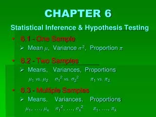
CHAPTER 6 Statistical Inference & Hypothesis Testing . 6.1 - One Sample Mean μ , Variance σ 2 , Proportion π 6.2 - Two Samples Means, Variances, Proportions μ 1 vs. μ 2 σ 1 2 vs. σ 2 2 π 1 vs. π 2 6.3 - Multiple Samples Means, Variances, Proportions

CHAPTER 6 Statistical Inference & Hypothesis Testing
E N D
Presentation Transcript
CHAPTER 6Statistical Inference & Hypothesis Testing 6.1 - One Sample Mean μ, Variance σ2, Proportion π 6.2 - Two Samples Means, Variances, Proportions μ1vs.μ2σ12vs.σ22π1vs.π2 6.3 - Multiple Samples Means, Variances, Proportions μ1, …, μkσ12, …,σk2π1, …, πk
CHAPTER 6Statistical Inference & Hypothesis Testing 6.1 - One Sample Mean μ, Variance σ2, Proportion π 6.2 - Two Samples Means, Variances, Proportions μ1vs.μ2σ12vs.σ22π1vs.π2 6.3 - Multiple Samples Means, Variances, Proportions μ1, …, μkσ12, …,σk2π1, …, πk
Example:Y = “$ Cost of a certain medical service” Assume Y is known to be normally distributed at each of k = 2 health care facilities (“groups”). Hospital: Y1 ~ N(μ1, σ1) Clinic: Y2 ~ N(μ2, σ2) • Null Hypothesis H0: μ1 = μ2, • i.e., μ1 – μ2= 0 • (“No difference exists.") • 2-sided test at significance level α = .05 • Data: Sample 1 ={667, 653, 614, 612, 604}; n1 = 5 Sample 2 ={593, 525, 520}; n2 = 3 NOTE: > 0 • Analysis via T-test(if equivariance holds): Point estimates “Group Means” “Group Variances” SS1 SS2 s2 = SS/df Pooled Variance The pooled variance is a weighted average of the group variances, using the degrees of freedom as the weights.
Example:Y = “$ Cost of a certain medical service” Assume Y is known to be normally distributed at each of k = 2 health care facilities (“groups”). Hospital: Y1 ~ N(μ1, σ1) Clinic: Y2 ~ N(μ2, σ2) • Null Hypothesis H0: μ1 = μ2, • i.e., μ1 – μ2= 0 • (“No difference exists.") • 2-sided test at significance level α = .05 • Data: Sample 1 ={667, 653, 614, 612, 604}; n1 = 5 Sample 2 ={593, 525, 520}; n2 = 3 NOTE: > 0 • Analysis via T-test(if equivariance holds): Point estimates “Group Means” “Group Variances” s2 = SS/df SSErr = 6480 Pooled Variance The pooled variance is a weighted average of the group variances, using the degrees of freedom as the weights. dfErr = 6 p-value = Reject H0 at α = .05 stat signif, Hosp > Clinic > 2 * (1 - pt(3.5, 6)) Standard Error [1] 0.01282634
R code: > y1 = c(667, 653, 614, 612, 604) > y2 = c(593, 525, 520) > > t.test(y1, y2, var.equal = T) Two Sample t-test data: y1 and y2 t = 3.5, df = 6, p-value = 0.01283 alternative hypothesis: true difference in means is not equal to 0 95 percent confidence interval: 25.27412 142.72588 sample estimates: mean of x mean of y 630 546 Formal Conclusion p-value < α = .05 Reject H0at this level. Interpretation The samples provide evidence that the difference between mean costs is (moderately) statistically significant, at the 5% level, with the hospital being higher than the clinic (by an average of $84).
k 1 2 Analysis of Variance (ANOVA) Alternate method ~ • Main Idea: Among several (k 2) independent, equivariant, normally-distributed “treatment groups”… “Total Variability” = “Variability between groups” + “Variability within groups” H0: = = = Null Hypothesis? HA:“At least one ‘treatment mean’ μi is significantly different from the others.
Example:Y = “$ Cost of a certain medical service” Assume Y is known to be normally distributed at each of k = 2 health care facilities (“groups”). Hospital: Y1 ~ N(μ1, σ1) Clinic: Y2 ~ N(μ2, σ2) • Null Hypothesis H0: μ1 = μ2, • i.e., μ1 – μ2= 0 • (“No difference exists.") • 2-sided test at significance level α = .05 • Data: Sample 1 ={667, 653, 614, 612, 604}; n1 = 5 Sample 2 ={593, 525, 520}; n2 = 3 ANOVA F-test NOTE: > 0 • (if equivariance holds): Point estimates “Group Means” 3 (546) 5 (630) “Grand Mean” The grand mean is a weighted average of the group means, using the sample sizes as the weights.
k 1 2 Analysis of Variance (ANOVA) Alternate method ~ • Main Idea: Among several (k 2) independent, equivariant, normally-distributed “treatment groups”… “Total Variability” = “Variability between groups” + “Variability within groups” H0: = = = HA:“At least one ‘treatment mean’ μi is significantly different from the others.
Example:Y = “$ Cost of a certain medical service” Assume Y is known to be normally distributed at each of k = 2 health care facilities (“groups”). Hospital: Y1 ~ N(μ1, σ1) Clinic: Y2 ~ N(μ2, σ2) • Null Hypothesis H0: μ1 = μ2, • i.e., μ1 – μ2= 0 • (“No difference exists.") • 2-sided test at significance level α = .05 • Data: Sample 1 ={667, 653, 614, 612, 604}; n1 = 5 Sample 2 ={593, 525, 520}; n2 = 3 ANOVA F-test • (if equivariance holds): Point estimates “Group Means” “Grand Mean” How far is the “total” sample from the grand mean?
Example:Y = “$ Cost of a certain medical service” Assume Y is known to be normally distributed at each of k = 2 health care facilities (“groups”). Hospital: Y1 ~ N(μ1, σ1) Clinic: Y2 ~ N(μ2, σ2) • Null Hypothesis H0: μ1 = μ2, • i.e., μ1 – μ2= 0 • (“No difference exists.") • 2-sided test at significance level α = .05 • Data: Sample 1 ={667, 653, 614, 612, 604}; n1 = 5 Sample 2 ={593, 525, 520}; n2 = 3 ANOVA F-test • (if equivariance holds): Point estimates “Group Means” “Grand Mean” SSTot = = 19710 dfTot = = 7 (5+3) –1
k 1 2 Analysis of Variance (ANOVA) Alternate method ~ • Main Idea: Among several (k 2) independent, equivariant, normally-distributed “treatment groups”… “Total Variability” = “Variability between groups” + “Variability within groups” H0: = = = Imagine zero variability within groups… How can we measure this?
k 1 2 Analysis of Variance (ANOVA) Alternate method ~ • Main Idea: Among several (k 2) independent, equivariant, normally-distributed “treatment groups”… “Total Variability” = “Variability between groups” + “Variability within groups” H0: = = = Imagine zero variability within groups… How can we measure this?
Example:Y = “$ Cost of a certain medical service” Assume Y is known to be normally distributed at each of k = 2 health care facilities (“groups”). Hospital: Y1 ~ N(μ1, σ1) Clinic: Y2 ~ N(μ2, σ2) • Null Hypothesis H0: μ1 = μ2, • i.e., μ1 – μ2= 0 • (“No difference exists.") • 2-sided test at significance level α = .05 • Data: Sample 1 ={667, 653, 614, 612, 604}; n1 = 5 Sample 2 ={593, 525, 520}; n2 = 3 {630, 630, 630, 630, 630} {546, 546, 546} ANOVA F-test • (if equivariance holds): Point estimates “Group Means” “Grand Mean” SSTot = = 19710 dfTot = = 7 (5+3) –1 SSTrt = dfTrt = = 1 = 13230 (2) –1 “The Clonemaster”
k 1 2 Analysis of Variance (ANOVA) Alternate method ~ • Main Idea: Among several (k 2) independent, equivariant, normally-distributed “treatment groups”… “Total Variability” = “Variability between groups” + “Variability within groups” H0: = = =
Example:Y = “$ Cost of a certain medical service” Assume Y is known to be normally distributed at each of k = 2 health care facilities (“groups”). Hospital: Y1 ~ N(μ1, σ1) Clinic: Y2 ~ N(μ2, σ2) • Null Hypothesis H0: μ1 = μ2, • i.e., μ1 – μ2= 0 • (“No difference exists.") • 2-sided test at significance level α = .05 • Data: Sample 1 ={667, 653, 614, 612, 604}; n1 = 5 Sample 2 ={593, 525, 520}; n2 = 3 ANOVA F-test • (if equivariance holds): Point estimates “Group Means” “Grand Mean” SSTot = = 19710 dfTot = = 7 (5+3) –1 SSTrt = dfTrt = = 1 = 13230 (2) –1 How far is each sample from its own group mean?
Example:Y = “$ Cost of a certain medical service” Assume Y is known to be normally distributed at each of k = 2 health care facilities (“groups”). Hospital: Y1 ~ N(μ1, σ1) Clinic: Y2 ~ N(μ2, σ2) • Null Hypothesis H0: μ1 = μ2, • i.e., μ1 – μ2= 0 • (“No difference exists.") • 2-sided test at significance level α = .05 • Data: Sample 1 ={667, 653, 614, 612, 604}; n1 = 5 Sample 2 ={593, 525, 520}; n2 = 3 ANOVA F-test • (if equivariance holds): Point estimates “Group Means” “Grand Mean” SSTot = = 19710 dfTot = = 7 (5+3) –1 SSTrt = dfTrt = = 1 = 13230 (2) –1 BUT… SSErr =
Example:Y = “$ Cost of a certain medical service” Assume Y is known to be normally distributed at each of k = 2 health care facilities (“groups”). Hospital: Y1 ~ N(μ1, σ1) Clinic: Y2 ~ N(μ2, σ2) • Null Hypothesis H0: μ1 = μ2, • i.e., μ1 – μ2= 0 • (“No difference exists.") • 2-sided test at significance level α = .05 • Data: Sample 1 ={667, 653, 614, 612, 604}; n1 = 5 Sample 2 ={593, 525, 520}; n2 = 3 NOTE: > 0 • Analysis via T-test(if equivariance holds): Point estimates “Group Means” “Group Variances” SS1 SS2 s2 = SS/df Pooled Variance The pooled variance is a weighted average of the group variances, using the degrees of freedom as the weights. RECALL…
Example:Y = “$ Cost of a certain medical service” Assume Y is known to be normally distributed at each of k = 2 health care facilities (“groups”). Hospital: Y1 ~ N(μ1, σ1) Clinic: Y2 ~ N(μ2, σ2) • Null Hypothesis H0: μ1 = μ2, • i.e., μ1 – μ2= 0 • (“No difference exists.") • 2-sided test at significance level α = .05 • Data: Sample 1 ={667, 653, 614, 612, 604}; n1 = 5 Sample 2 ={593, 525, 520}; n2 = 3 NOTE: > 0 • Analysis via T-test(if equivariance holds): Point estimates “Group Means” “Group Variances” s2 = SS/df SSErr = 6480 Pooled Variance The pooled variance is a weighted average of the group variances, using the degrees of freedom as the weights. dfErr = 6 RECALL…
Example:Y = “$ Cost of a certain medical service” Assume Y is known to be normally distributed at each of k = 2 health care facilities (“groups”). Hospital: Y1 ~ N(μ1, σ1) Clinic: Y2 ~ N(μ2, σ2) • Null Hypothesis H0: μ1 = μ2, • i.e., μ1 – μ2= 0 • (“No difference exists.") • 2-sided test at significance level α = .05 • Data: Sample 1 ={667, 653, 614, 612, 604}; n1 = 5 Sample 2 ={593, 525, 520}; n2 = 3 ANOVA F-test • (if equivariance holds): Point estimates “Group Means” “Grand Mean” SSTot = = 19710 dfTot = = 7 (5+3) –1 SSTrt = dfTrt = = 1 = 13230 (2) –1 SSErr =
Example:Y = “$ Cost of a certain medical service” Assume Y is known to be normally distributed at each of k = 2 health care facilities (“groups”). Hospital: Y1 ~ N(μ1, σ1) Clinic: Y2 ~ N(μ2, σ2) • Null Hypothesis H0: μ1 = μ2, • i.e., μ1 – μ2= 0 • (“No difference exists.") • 2-sided test at significance level α = .05 • Data: Sample 1 ={667, 653, 614, 612, 604}; n1 = 5 Sample 2 ={593, 525, 520}; n2 = 3 ANOVA F-test • (if equivariance holds): Point estimates “Group Means” “Grand Mean” SSTot = = 19710 dfTot = = 7 (5+3) –1 SSTrt = dfTrt = = 1 = 13230 (2) –1 = 6480 SSErr = dfErr = = 6 (5+3) –2 SSTot = SSTrt + SSErr dfTot = dfTrt + dfErr
SSTot = SSTrt + SSErr dfTot = dfTrt + dfErr Tot Err Trt ANOVA Table 12.25 1–pf(12.25, 1, 6) F-table: comp w/ α Note: This is also SSTot = SSTrt + SSErr dfTot = dfTrt + dfErr
SSTot = SSTrt + SSErr dfTot = dfTrt + dfErr Tot Err Trt ANOVA Table 12.25 13230 1–pf(12.25, 1, 6) F-table: comp w/ α 19710 Thus, the treatment accounts for = 67.1% of the total variability in the response Y.
R code: # ANOVA FOR UNBALANCED DESIGN > y1 = c(667, 653, 614, 612, 604) > y2 = c(593, 525, 520) > > Data = data.frame( + Y = c(y1, y2), + X = factor(rep(c("y1", "y2"), times = c(length(y1), length(y2)))) + ) > > var.test(Y ~ X, data = Data) # EQUIVARIANCE? F test to compare two variances data: Y by X F = 0.4741, num df = 4, denomdf = 2, p-value = 0.4738 alternative hypothesis: true ratio of variances is not equal to 1 95 percent confidence interval: 0.01208057 5.04920249 sample estimates: ratio of variances 0.4741431
R code: • # ANOVA FOR UNBALANCED DESIGN • > out = aov(Y ~ X, data = Data) • > anova(out) • Analysis of Variance Table • Response: Y • Df Sum Sq Mean Sq F value Pr(>F) • X 1 13230 13230 12.25 0.01283 * • Residuals 6 6480 1080 • --- • Signif. codes: 0 ‘***’ 0.001 ‘**’ 0.01 ‘*’ 0.05 ‘.’ 0.1 ‘ ’ 1 • Note: Vis-à-vis T-test vs. F-test, • p-value is the same using either method (.01283), since the sample is unchanged! • The square of the Tdf -score (3.5) is equal to the F1, df -score (12.25). • (Recall that the square of the Z-score is equal to the -score.)
k 1 2 Analysis of Variance (ANOVA) Alternate method ~ • Main Idea: Among several (k 2) independent, equivariant, normally-distributed “treatment groups”… MODEL ASSUMPTIONS? H0: = = =
k 1 2 Analysis of Variance (ANOVA) Alternate method ~ • Main Idea: Among several (k 2) independent, equivariant, normally-distributed “treatment groups”… • Equivariance can be tested via very similar “two variances” F-test in 6.2.2 (but this is very sensitive to normality assumption), or others. If violated, can extend Welch Test for two means. H0: = = =
k 1 2 Analysis of Variance (ANOVA) Alternate method ~ • Main Idea: Among several (k 2) independent, equivariant, normally-distributed “treatment groups”… • Normality can be tested via usual methods. • If violated, use nonparametricKruskal-Wallis Test. H0: = = =
k 1 2 Analysis of Variance (ANOVA) Alternate method ~ • Main Idea: Among several (k 2) independent, equivariant, normally-distributed “treatment groups”… • Extensions of ANOVA for data in matched “blocks” designs, repeated measures, multiple factor levels within groups, etc. H0: = = =
k 1 2 Analysis of Variance (ANOVA) Alternate method ~ • Main Idea: Among several (k 2) independent, equivariant, normally-distributed “treatment groups”… • How to identify significant group(s)? Pairwise testing, with correction (e.g., Bonferroni) for spurious significance. • Example:k = 5 groups result in 10 such tests, so let each α* = α / 10. H0: = = =