8.3 Testing the Difference Between Means (Dependent Samples)
8.3 Testing the Difference Between Means (Dependent Samples). Statistics Mrs. Spitz Spring 2009. Objectives/Assignment. How to decide whether two samples are independent or dependent How to perform a t-test to test the mean of the differences for a population of paired data


8.3 Testing the Difference Between Means (Dependent Samples)
E N D
Presentation Transcript
8.3 Testing the Difference Between Means (Dependent Samples) Statistics Mrs. Spitz Spring 2009
Objectives/Assignment • How to decide whether two samples are independent or dependent • How to perform a t-test to test the mean of the differences for a population of paired data Assignment: 8.3 pp. 395-399 #1-16
Independent and Dependent Samples • In Sections 8.1 and 8.2, you studied two-sample hypothesis tests in which the samples were independent. In this section, you will learn how to perform two-sample hypothesis tests using dependent samples
Definition • Two samples are independent if the sample selected from one population is not related to the sample selected from the second population. The two samples are dependent if each member of one sample corresponds to a member of the other sample. Dependent samples are also called paired samples or matched samples.
Ex. 1a: Independent and Dependent Samples • Classify each pair of samples as independent or dependent: Sample 1: Resting heart rates of 35 individuals before drinking coffee. Sample 2: Resting heart rates of the same individuals after drinking two cups of coffee.
Ex. 1: Independent and Dependent Samples Sample 1: Resting heart rates of 35 individuals before drinking coffee. Sample 2: Resting heart rates of the same individuals after drinking two cups of coffee. These samples are dependent. Because the resting heart rates of the same individuals were taken, the samples are related. The samples can be paired with respect to each individual.
Ex. 1b: Independent and Dependent Samples • Classify each pair of samples as independent or dependent: Sample 1: Test scores for 35 statistics students Sample 2: Test scores for 42 biology students who do not study statistics
Ex. 1b: Independent and Dependent Samples Sample 1: Test scores for 35 statistics students Sample 2: Test scores for 42 biology students who do not study statistics These samples are independent. It is not possible to form a pairing between the members of samples—the sample sizes are different and the data represent test scores for different individuals.
Note: Dependent samples often involve identical twins, before and after results for the same person or object, or results of individuals matched for specific characteristics.
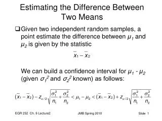
The t-Test for the Difference Between Means • In 8.1 and 8.2, you were using the test statistic, (the difference in the means of two samples). To perform a two-sample hypothesis test with dependent samples, you will use a different technique. You will first find the difference for each data pair, . The test statistic is the mean of these differences,
To conduct the test, the following conditions are required: • The samples must be dependent (paired) and randomly selected. • Both populations must be normally distributed. If these two requirements are met, then the sampling distribution for , the mean of the differences of the paired data entries in the dependent samples,
To conduct the test, the following conditions are required: • has a t-distribution with n – 1 degrees of freedom, where n is the number of data pairs.
The following symbols are used for the t-test for d. Although formulas are given for the mean and standard deviation of differences, we suggest you use a technology tool to calculate these statistics.
Because the sampling distribution for is a t-distribution, you can use a t-test to test a claim about the mean of the differences for a population of paired data. STUDY TIP: If n > 29, use the last row (∞) in the t-distribution table.
Ex. 2: The t-Test for the Difference Between Means • A golf club manufacturer claims that golfers can lower their score by using the manufacturer’s newly designed golf clubs. Eight golfers are randomly selected and each is asked to give his or her most recent score. After using the new clubs for one month, the golfers are again asked to give their most recent scores. The scores for each golfer are given in the next slide. Assuming the golf scores are normally distributed, is there enough evidence to support the manufacturer’s claim at = 0.10?
The claim is that “golfers can lower their scores.” In other words, the manufacturer claims that the score using the old clubs will be greater than the score using the new clubs. Each difference is given by: d = (old score) – (new score) The null and alternative hypotheses are Ho: d 0 and Ha: d > 0 (claim)
Because the test is a right-tailed test, = 0.10, and d.f. = 8 – 1 = 7, the critical value for t is 1.415. The rejection region is t > 1.415. Using the table below, you can calculate and sd as follows:
Using the t-test, the standardized test statistic is: • The graph below shows the location of the rejection region and the standardized test statistic, t. Because t is in the rejection region, you should decide to reject the null hypothesis. There is not enough evidence to support the golf manufacturer’s claim at the 10% level The results of this test indicate that after using the new clubs, golf scores were significantly lower.
Ex. 3: The t-Test for the Difference Between Means • A state legislator wants to determine whether her voter’s performance rating (0-100) has changed from last year to this year. The following table shows the legislator’s performance rating for the same 16 randomly selected voters for last year and this year. At = 0.01, is there enough evidence to conclude that the legislator’s performance rating has changed? Assume the performance ratings are normally distributed.
If there is a change in the legislator’s rating, there will be a difference between “this year’s” ratings and “last year’s) ratings. Because the legislator wants to see if there is a difference, the null and alternative hypotheses are: Ho: d = 0 and Ha: d 0 (claim)
Because the test is a tw0-tailed test, = 0.01, and d.f. = 16 – 1 = 15, the critical values for t are 2.947. The rejection region are t < -2.947 and t > 2.947.
Using the t-test, the standardized test statistic is: • The graph shows the location of the rejection region and the standardized test statistic, t. Because t is not in the rejection region, you should fail to reject the null hypothesis at the 1% level. There is not enough evidence to conclude that the legislator’s approval rating has changed.
If you prefer to use a technology tool for this type of test, enter the data in two columns and form a third column in which you calculate the difference for each pair. You can now perform a one-sample t-test on the difference column as shown in Chapter 7. Stat|Edit|enter data Subtract L1 – L2 = in L3. STAT|Tests|t-test Data = 0 List: L3 Freq: 1 0 Calculate Using Technology
Stat|Edit|enter data Subtract L1 – L2 = in L3. STAT|Tests|t-test Data = 0 List: L3 Freq: 1 0 Calculate 0 T = 1.369 (standardized test statistic) P = don’t worry about it X bar = 3.3125 – same as d bar. Sx = 9.68 which is Sd I find it easy to draw and enter the data into the curve part so I can visually see the rejection region. You will need to answer “reject” or “fail to reject” and answer whether or not there is enough evidence at whatever level given. Using Technology