Download

1 / 28
300 likes | 663 Vues
8.1 Testing the Difference Between Means (Large Independent Samples). Statistics Mrs. Spitz Spring 2009. Objectives/Assignment. An introduction to two-sample hypothesis testing for the difference between two population parameters.

E N D
8.1 Testing the Difference Between Means (Large Independent Samples) Statistics Mrs. Spitz Spring 2009
Objectives/Assignment • An introduction to two-sample hypothesis testing for the difference between two population parameters. • How to perform a two-sample z-test for the difference between two means 1 and 2, using large independent samples • Assignment: pp. 373-378 #1-26
An overview of Two-Sample Hypothesis Testing • In Chapter 7, you studied methods for testing a claim about the value of a population parameter. In this chapter, you will learn how to test a claim comparing parameters from two populations. • For instance, suppose you are developing a marketing plan for an Internet service provider and want to determine whether there is a difference in the amount of time male and female college students spen online each day.
An overview of Two-Sample Hypothesis Testing • The only way you could conclude with certainty that there is a difference is to take a census of all college students, calculate the mean daily times male students and female students spend time online, and find the difference. Of course if it not practical to take such a census. However, you can still determine with some degree of certainty if such a difference exists.
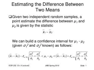
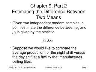
An overview of Two-Sample Hypothesis Testing • You can begin by assuming that there is no difference in the mean times of the two populations. That is 1 – 2 = 0. Then by taking a random sample from each population, and using the resulting two-sample test statistic , you can perform a two-sample hypothesis test. Suppose you obtain the following results.
The graph on the next slide shows the sampling distribution of for many similar samples taken from each population. From the graph, you can see that it is quite unlikely to obtain sample means that differ by 4 minutes when the actual difference is 0. The difference of the sample means is more than 2.5 standard errors from the hypothesized difference of 0!
So, you can conclude there is a significant difference in the amount of time male college students and female college students spend online each day. • It is important to remember that when you perform a two-sample hypothesis test, you are testing a claim concerning the difference between the parameters in two populations, not the values of the parameters themselves.
Null/Alternative Hypothesis • To write a null and an alternative hypothesis for a two-sample hypothesis test, translate the claim made about the population parameters from a verbal statement to a mathematical statement. Then, write its complementary statement. For instance, if the claim is about two population parameters, 1 and 2, then some possible pairs of null and alternative hypotheses are:
Study Tip: • You can also write the null and alternative hypotheses as follows.
Two-Sample z-test for the Difference Between Means • In the remainder of this section, you will learn how to perform a z-test for the difference between two population means 1 and 2. To perform such a test, two conditions are necessary. 1. The samples must be independent. Two samples are independent if the sample selected from one population is not related to the sample selected from the second population. (more in 8.3) 2. Each sample size must be at least 30 or, if not, each population must have a normal distribution with a known standard deviation.
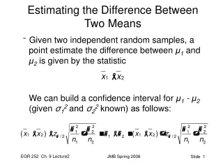
Two-Sample z-test for the Difference Between Means • If these requirements are met, then the sampling distribution for (the difference of the sample means) is a normal distribution with mean and standard deviation of
And Notice that the variance of the sampling distribution is the sum of the variances of the individual sampling distributions for
Two-Sample z-test for the Difference Between Means • Because the sampling distribution for is a normal distribution, you can use the z-test to test the difference between two population means 1 and 2. Notice that the standardized test statistic takes the form of:
If the null hypothesis states that 1 = 2, then the expression 1 – 2 is equal to 0 in the preceding test.
Ex. 1: A Two-Sample z-test for the Difference Between Means • An advertising executive claims that there is a difference in the mean household income for credit card holders of Visa Gold and of MasterCard Gold. The results of a random survey of 100 customers from each group are shown. The two samples are independent. Do the results support the executive’s claim? Use = 0.05..
Solution: • You want to test the claim that there is a difference in the mean household incomes for Visa Gold and MasterCard Gold credit card holders. So, the null and alternative hypotheses are: Ho: 1 = 2 and Ha: 1 2(Claim)
Solution: • Because the test is a two-tailed test and the level of significance is = 0.05, you look up the critical values and find they are -1.96 and 1.96. The rejection regions are z < -1.96 and z > 1.96. Because both samples are large, s1 and s2 are used to calculate the standard error.
Solution: • Using the z-test, the standardized test statistic is:
Solution: • The graph at the left shows the location of the rejection regions and the standardized test statistic, z. Because z Is not in the rejection region, you should fail to reject the null hypothesis. At the 5% level, there is not enough evidence to conclude that there is a significant difference in the mean household incomes of Visa Gold and MasterCard Gold credit card holders.
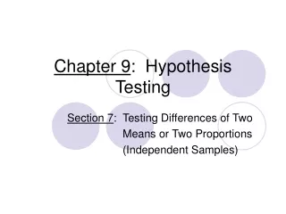
Ex. 2: Using Technology to Perform a Two-Sample z-test • The American Automobile Association (AAA) claims that the average daily cost for meals and lodging when vacationing in Texas is less than the same average costs when visiting Washington state. The table on the next slide shows the results of a survey of vacationers in each state. At = 0.01, is there enough evidence to support the claim? Ho: 1≥ 2 and Ha: 1 2(Claim)
Note: Texas is population 1 and Washington is population 2 • The first two displays show how to set up the hypothesis test using a TI-83. The remaining displays show the possible results depending on whether you select “Calculate” or “Draw.” • STAT • Arrow to TESTS • Choose 3: 2-SampZTest • Arrow to DATA and Enter • Enter as shown on the right • Arrow to < 2 and Arrow to • Calculate then Enter
To Draw 2-sample z • The first two displays show how to set up the hypothesis test using a TI-83. The remaining displays show the possible results depending on whether you select “Calculate” or “Draw.” • STAT • Arrow to TESTS • Choose 3: 2-SampZTest • Arrow down to • DRAW then Enter
Reject or Fail to Reject? • Because the test is a left-tailed test and = 0.01, the rejection region is z < -2.33. The standardized test statistic, z -2.12, is Not in the rejection region, so you should fail to reject the null hypothesis. At the 1% level, there is not evidence to support the American Automobile Association’s claim.
One more on the calculator • The American Automobile Association claims that the average daily meal and lodging costs while vacationing in Florida are greater than the same costs while vacationing in Maryland. The table shows the results of a survey of vacationers in each state. At = 0.05, is there enough evidence to support the claim? 1. Use a calculator to find the test statistic or P-value. 2. Determine whether the test statistic is in the rejection region or compare the P-value to the level of significance, . 3. Make a decision.
Solution: • Z = 3.634, p = 0.000014 • Rejection region is z > 1.645 or p-value < 0.05 = (Look up value closest – or use that table from Chapter 6 with the z-values given) • Reject Ho because 3.634 is greater than 1.645 and because 0.00014 is less than 0.05.
Upcoming • Last day for the quarter is March 11 • Monday 2/23 – Notes 8.1 • Tuesday 2/24 – work on 8.1 work • Wednesday 2/25– Notes 8.2 • Thursday 2/26 – Work on 8.2 • Friday 2/27 – Notes 8.3 • Monday 3/2 – Work on 8.3 • Tuesday 3/3 – Notes 8.4 • Wednesday 3/4 – Work on 8.4 • Thursday/Fri 3/5-6 – Review for Chapter 8 Exam • Monday 3/9 – Chapter 8 TEST – Everyone must be here for the exam. I am tired of people flaking out. There is no excuse for it.