Download
1 / 55
590 likes | 1.02k Vues
Independent Samples T-Test of Population Means. Key Points about Statistical Test Sample Homework Problem Solving the Problem with SPSS Logic for Independent Samples T-Test of Population Means Power Analysis. Independent Samples T-Test: Purpose.

E N D
Independent Samples T-Test of Population Means Key Points about Statistical Test Sample Homework Problem Solving the Problem with SPSS Logic for Independent Samples T-Test of Population Means Power Analysis
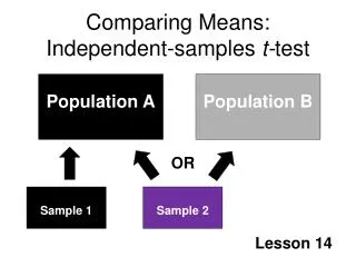
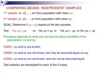
Independent Samples T-Test: Purpose • Purpose: test whether or not the populations represented by the two samples have a different mean • Examples: • Social work students have higher GPA’s than nursing students • Social work students volunteer for more hours per week than education majors • UT social work students score higher on licensing exams than graduates of Texas State University
Independent Samples T-Test: Hypotheses • Hypotheses: • Null: mean of population 1 = mean of population 2 Versus • Research: mean of population 1 < mean of population 2 • Research: mean of population 1 ≠ mean of population 2 • Research: mean of population 1 > mean of population 2 • Decision: • Reject null hypothesis if pSPSS ≤ alpha (≠ relationship) • Reject null hypothesis if pSPSS÷2 ≤ alpha (< or > relationship)
Independent Samples T-Test: Assumptions and Requirements • Variable is interval level (ordinal with caution) • Variable is normally distributed • Acceptable degree of skewness and kurtosis or • Using the Central Limit Theorem (30+ in each group) • The variance of the two groups is not different (if different, use alternative formula)
Independent Samples T-Test: Effect Size • Cohen’s d measures difference in means in standard deviation units. • Cohen’s d = difference in population means population standard deviation • Interpretation: • small: d = .20 to .50 • medium: d = .50 to .80 • large: d = .80 and higher
Independent Samples T-Test: APA Style • An independent samples T-test is presented the same as the one-sample t-test: t(75) = 2.11, p = .02 (one –tailed), d = .48 • Example: Survey respondents who were employed by the federal, state, or local government had significantly higher socioeconomic indices (M = 55.42, SD = 19.25) than survey respondents who were employed by a private employer (M = 47.54, SD = 18.94) , t(255) = 2.363, p = .01 (one-tailed). Degrees of freedom Value of statistic Significance of statistic Include if test is one-tailed Effect size if available
Homework problems: Independent Samples T-Test of Population Means This problem uses the data set GSS2000R.Sav to compare the average score on the variable "highest year of school completed" [educ] for groups of survey respondents defined by the variable "governmental employment" [wrkgovt]. Using an independent samples t-test with an alpha of .05, is the following statement true, true with caution, false, or an incorrect application of a statistic? Survey respondents who were employed by the federal, state, or local government completed significantly more years of school (M = 13.97, SD = 3.27) than survey respondents who were employed by a private employer (M = 13.07, SD = 2.84) . • True • True with caution • False • Incorrect application of a statistic This is the general framework for the problems in the homework assignment on “Independent Samples T-Test of Population Means.” The description is similar to findings one might state in a research article.
Homework problems: Independent Samples T-Test - Data set, variables, and sample This problem uses the data set GSS2000R.Sav to compare the average score on the variable "highest year of school completed" [educ]for groups of survey respondents defined by the variable "governmental employment" [wrkgovt]. Using an independent samples t-test with an alpha of .05, is the following statement true, true with caution, false, or an incorrect application of a statistic? Survey respondents who were employed by the federal, state, or local government completed significantly more years of school (M = 13.97, SD = 3.27) than survey respondents who were employed by a private employer (M = 13.07, SD = 2.84) . • True • True with caution • False • Incorrect application of a statistic • The first paragraph identifies: • The data set to use, e.g. GSS2000R.Sav • The groups that will be compared in the analysis • The variable compared in the t-test • Thealpha level to use for the hypothesis test
Homework problems: Independent Samples T-Test - Specifications This problem uses the data set GSS2000R.Sav to compare the average score on the variable "highest year of school completed" [educ] for groups of survey respondents defined by the variable "governmental employment" [wrkgovt]. Using an independent samples t-test with an alpha of .05, is the following statement true, true with caution, false, or an incorrect application of a statistic? Survey respondents who were employed by the federal, state, or local governmentcompleted significantly more years of school(M = 13.97, SD = 3.27) than survey respondents who were employed by a private employer (M = 13.07, SD = 2.84) . • True • True with caution • False • Incorrect application of a statistic • The second paragraph specifies: • The sample means and standard deviation for the groups being compared • The relationship for deriving the research hypothesis
Homework problems: Independent SamplesT- Test - Choosing an answer The answer to a problem will be True if the t-test supports the finding in the problem statement. The answer to a problem will be True with caution if the t-test supports the finding in the problem statement, but the dependent variable is ordinal level. This problem uses the data set GSS2000R.Sav to compare the average score on the variable "highest year of school completed" [educ] for groups of survey respondents defined by the variable "governmental employment" [wrkgovt]. Using an independent samples t-test with an alpha of .05, is the following statement true, true with caution, false, or an incorrect application of a statistic? Survey respondents who were employed by the federal, state, or local government completed significantly more years of school (M = 13.97, SD = 3.27) than survey respondents who were employed by a private employer (M = 13.07, SD = 2.84) . • True • True with caution • False • Incorrect application of a statistic • The answer to a problem will Incorrect application of a statistic if • the t-test violates the level of measurement requirement, i.e. the dependent variable is nominal • the assumption of normality of the dependent variable is violated and the central limit theorem doesn’t apply • the independent variable is not dichotomous The answer to a problem will be False if the t-test does not support the finding in the problem statement.
Solving the problem with SPSS: Identifying numeric codes for groups - 1 Our first task in SPSS is to identify the numeric codes for the groups that SPSS will require us to specify. The problem statement tells us “This problem uses the data set GSS2000R.Sav to compare the average score on the variable "highest year of school completed" [educ] for groups of survey respondents defined by the variable "governmental employment" [wrkgovt].” Select the Variables… command from the Utilities menu. NOTE: in our problems we required that the grouping, or independent variable, be dichotomous, because there are other statistical tests to use when there are more than two groups. SPSS does not require the independent variable to be dichotomous, but it does require that you enter the numeric codes for the two groups (possibly out of a larger number of groups) that you wish to compare.
Solving the problem with SPSS: Identifying numeric codes for groups - 2 Scroll through the list of variables until you see wkgovt. Click on wkgovt and the information for the variable appears in the panel to the right. Click on Close to dismiss the dialog box. The Variable Information panel shows us the text labels that the creator of the data set assigned to each of the possible numeric responses for this variable. The numeric codes for the groups we want to compare are: 1 (GOVERNMENT) and 2 (PRIVATE). This remaining numeric codes represent missing data: 0 (NAP), 8 (DK), and 9 (NA).
Solving the problem with SPSS:Level of measurement Statistical tests of means require that the dependent variable be interval level. "Highest year of school completed" [educ] is interval level, satisfying the requirement. In our analyses, we will allow the dependent variable to be ordinal , which violates this requirement in the strictest interpretation of level of measurement. However, since the research literature often computes means for ordinal level data, especially scaled measures, we will follow the convention of applying interval level statistics to ordinal data. Since all analysts may not agree with this convention, a caution is added to any true findings.
Solving the problem with SPSS: Evaluating normality - 1 The independent samples t-test uses the t-distribution for the probability of the test statistic. To obtain accurate probabilities, the variable must follow a normal distribution. We will generate descriptive statistics to evaluate normality. Select the Descriptive Statistics > Descriptives… command from the Analysis menu.
Solving the problem with SPSS: Evaluating normality - 2 First, move the variable we will use in the t-test, educ, to the Variable(s) list box. Second, click on the Options… button to select the statistics we want.
Solving the problem with SPSS: Evaluating normality - 3 First, in addition to the statistics, SPSS has checked by default, mark the Kurtosis and Skewness check boxes on the Distribution panel. Second, click on the Continue button to close the dialog box.
Solving the problem with SPSS: Evaluating normality - 4 Click on the OK button to obtain the output.
Solving the problem with SPSS: Evaluating normality - 5 "Highest year of school completed" [educ] did not satisfy the criteria for a normal distribution. The skewness of the distribution (-.137) was between -1.0 and +1.0, but the kurtosis of the distribution (1.246) fell outside the range from -1.0 to +1.0. Having failed the normality requirement using this criteria, we will see if we can apply the central limit theorem.
Solving the problem with SPSS: The independent-samples t-test - 1 The number of cases in each group is part of the output for the independent samples t-test, so we will go ahead and compute that test to continue addressing the issue of normality. Select Compare Means > Independent-Samples T Test… from the Analyze menu.
Solving the problem with SPSS: The independent-samples t-test - 2 First, move the dependent variable educ to the Test Variable(s) list box. Second, move the independent variable wkgovt to the Grouping Variable text box. Note that SPSS lists two question marks after the variable name and activates the Define Groups… button as its clue for what it wants us to do next. Click on the Define Groups button.
Solving the problem with SPSS: The independent-samples t-test - 3 First, type in the numeric codes for the groups in the wkgovt variable that we looked up at the beginning of the problem. Second, click on the Continue button to close the dialog box.
Solving the problem with SPSS: The independent-samples t-test - 4 Click on the OK button to close the dialog box. Note that SPSS has replaced the question marks after the variable name with the numeric codes we typed in.
Solving the problem with SPSS: Evaluating normality with the central limit theorem - 6 Since survey respondents who were employed by the federal, state, or local government had 38 cases and survey respondents who were employed by a private employer had 217 cases, the assumption of normality was satisfied by the Central Limit Theorem which required both groups to have 30 or more cases. If we are unable to establish normality either by the distribution or by the central limit theorem, the t-test would not be an appropriate statistic.
Solving the problem with SPSS:Evaluating equality of group variances - 1 The independent-samples t-test assumes that the variances of the dependent variable for both groups are equal in the population. This assumption is evaluated with Levene's Test for Equality of Variances. The null hypothesis for this test states that the variance for both groups are equal. The desired outcome for this test is to fail to reject the null hypothesis, which demonstrates equality. The probability associated with Levene's Test for Equality of Variances (.161) is greater than alpha (.05), indicating that the 'Equal variances assumed' formula for the independent samples t-test should be used for the analysis.
Solving the problem with SPSS:Evaluating equality of group variances - 2 Since we failed to reject the hypothesis for Levene’s test, the 'Equal variances assumed' formula for the independent samples t-test should be used for the analysis. Had the probability associated with Levene’s test been less than the alpha level, we would have used the statistics for the ‘Equal variances not assumed’ row in the table.
Solving the problem with SPSS: Answering the question - 1 The finding we are trying to verify is: Survey respondents who were employed by the federal, state, or local government completed significantly more years of school (M = 13.97, SD = 3.27) than survey respondents who were employed by a private employer (M = 13.07, SD = 2.84) . Our first task is to make certain we have solved the right problem. Second, we verify that the mean and standard deviations for the groups match the problem statement. First, we check to make certain we have the correct groups in the output.
Solving the problem with SPSS: Answering the question - 2 The finding we are trying to verify is: Survey respondents who were employed by the federal, state, or local government completed significantly more years of school (M = 13.97, SD = 3.27) than survey respondents who were employed by a private employer (M = 13.07, SD = 2.84) . Since the problem states that the mean for one group is significantly higher than the mean of the other group, the research hypothesis is a one-tailed test. We divide the SPSS 2-tailed significance (.080) in half and make our decision about the null hypothesis by comparing p = .04 to alpha = .05.
Solving the problem with SPSS: Answering the question - 3 The answer to the question is True. We can include the t-test results in our statement of the finding: Survey respondents who were employed by the federal, state, or local government completed significantly more years of school (M = 13.97, SD = 3.27) than survey respondents who were employed by a private employer (M = 13.07, SD = 2.84) , t(255) = 1.761, p = .04 (one-tailed).
Logic for independent-samples t-test:Level of measurement Measurement level of independent variable? Dichotomous Interval/ordinal/nominal Measurement level of dependent variable? Inappropriate application of a statistic Nominal/ Dichotomous Interval/ordinal Strictly speaking, the test requires an interval level variable. We will allow ordinal level variables with a caution. Inappropriate application of a statistic
Logic for independent-samples t-test:Assumption of normality Number of cases in both groups is at least 30? Skewness and Kurtosis between -1.0 and +1.0? No No Inappropriate application of a statistic Yes Yes
Logic for independent-samples t-test:Assumption of equality of variances Probability for Levene test of equality of population variances less than or equal to alpha? Yes No Use ‘Equal variances not assumed’ Use ‘Equal variances assumed’
Logic for independent-samples t-test:Means and standard deviations correct Mean and standard deviation of both variables are correct? No Yes False
Logic for independent-samples t-test: Decision about null hypothesis One-tailed or two-tailed test? Two-tailed One-tailed Divide two-tailed significance by 2 Probability for t-test less than or equal to alpha? Yes No Add caution for ordinal dependent variable. True False
Power Analysis: Independent-samples T-test Problem that was False This problem uses the data set GSS2000R.Sav to compare the average score on the variable "number of hours worked in the past week" [hrs1] for groups of survey respondents defined by the variable "self-employment" [wrkslf]. Using an independent samples t-test with an alpha of .05, is the following statement true, true with caution, false, or an incorrect application of a statistic? Survey respondents who were self-employed worked significantly longer hours in the past week (M = 42.04, SD = 13.86) than survey respondents who were working for someone else (M = 40.55, SD = 12.46) . 1 True 2 True with caution 3 False 4 Incorrect application of a statistic The answer to this problem was false because the probability for the t-test was .29 (one-tailed), greater than the alpha of 0.05. We can conduct a post-hoc power analysis to determine what number of cases would have been sufficient to have a better opportunity to find a statistically significant difference.
Power Analysis: Statistical Results for False Independent-samples T-test - 1 The answer to the problem was false because the one-tailed significance was p = .29 (.583 ÷ 2), greater than the alpha of .05.
Power Analysis: Statistical Results for False Independent-samples T-test - 2 To calculate the effect size, and corresponding power, for this problem, we need a pooled estimate of the standard deviation for the two groups. SamplePower will calculate that for us, we will enter the sample sizes, means, and standard deviations for the two groups in SamplePower.
Access to SPSS’s SamplePower Program The UT license for SPSS does not include SamplePower, the SPSS program for power analysis. However, the program is available on the UT timesharing server. Information about access this program is available at this site.
Power Analysis for Independent-samples T-test - 1 In the SamplePower program on the ITS Timesharing Systems, select the New… command from the File menu.
Power Analysis for Independent-samples T-test - 2 First, select the Means tab to access the tests for means. Third, click on the Ok button to enter the specific values for our problem. Second, since we want to enter the means for our two groups, select the option button for t-test for 2 (independent) groups with common variance (Enter means)
Power Analysis for Independent-samples T-test – 3 I want to my entries to display two decimal places, instead of the default of 1, so I click on the Decimals displayed tool button.
Power Analysis for Independent-samples T-test – 4 First, click the up arrow button on the spinner for Decimals for data entry until 2 appears. Second, click on the OK button to close the dialog box.
Power Analysis for Independent-samples T-test - 5 SPSS sets the default test to a two-tailed test with an alpha of .05. Since our test was a one-tailed test with an alpha of .05, we click on the text specified as the SPSS default.
Power Analysis for Independent-samples T-test - 6 First, click on the 1 Tailed option on the Tails panel. Second, click on the Ok button to change the test specifications.
Power Analysis for Independent-samples T-test - 7 • We enter the values from the SPSS output from the independent-samples t-test for the Population 1 group: • 42.04 for Population Mean • 13.86 for Standard Deviation • 26 for the N Per Group • Note that SPSS fills in the standard deviation and N Per Group numbers for Population 2 with the same values.
Power Analysis for Independent-samples T-test – 8 First, enter the population mean for the second group, 40.55. When we click on the box to change the Standard Deviation, this message appears. Since the standard deviation for our two groups is not the same, we click on the Yes button.
Power Analysis for Independent-samples T-test – 9 We are now able to enter the standard deviation for the second group, 12.46.
Power Analysis for Independent-samples T-test – 10 When we click on the box to change the N Per Group for the second group, this message box below appears. Since the number of cases for our two groups is not the same, we click on the Yes button.
Power Analysis for Independent-samples T-test - 11 We are now able to enter the N Per Group for the second group, 145. Having entered the values for the two groups, we now click on the Compute button.
Power Analysis for Independent-samples T-test - 12 SamplePower tells us that our power to obtain statistical significance was 14%, translating to a possible successful outcome 1 in 7 tries.
Power Analysis for Independent-samples T-test – 13 With the mean difference of 1.49 and a pooled standard deviation of 12.68, we can use a calculator to compute the effect size of .12 (Cohen’s d), about half of what would be typically characterized as a small effect. Suppose, however, that even a very small effect of this size had important consequences. We can ask ourselves how large would the sample need to have been in order to find a statistically significant effect.