Independent Samples t-test
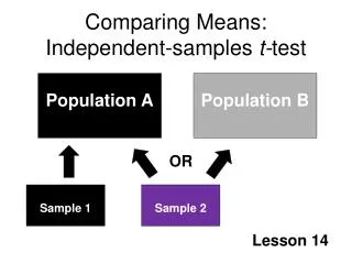
Independent Samples t-test. Mon, Apr 12 th. t Test for Independent Means. Comparing two samples e.g., experimental and control group Scores are independent of each other Focus on differences betw 2 samples, so comparison distribution is: Distribution of differences between means.

Independent Samples t-test
E N D
Presentation Transcript
Independent Samples t-test Mon, Apr 12th
t Test for Independent Means • Comparing two samples • e.g., experimental and control group • Scores are independent of each other • Focus on differences betw 2 samples, so comparison distribution is: • Distribution of differences between means
Hypotheses • Ho: or 1 - 2 = 0 (no group difference) or 1 = 2 • Ha = 1 - 2 not = 0 (2 tailed) or 1 - 2 > or < 0 (if 1-tailed) • If null hypothesis is true, the 2 populations (where we get sample means) have equal means • Compare T obs to T critical (w/Df= N-2) • If |Tobs| > |T crit| Reject Null
Pooled Variance • T observed will use concept of pooled variance to estimate standard error: • Assume the 2 populations have the same variance, but sample variance will differ… • so pool the sample variances to estimate pop variance • Then standard error used in denom of T obs • Note – I’ll show you 2 approaches (you decide which to use based on what data is given to you)
Finding Estimated Standard Error using SS (lab approach) • Pooled variance (S2p) S2p = (SS1 + SS2) / df1 + df2 Where, df1 = N1-1 and df2= N2-1 and SS1 and SS2 are given to you • Then use this to estimate standard error: (S xbar 1 –xbar2) = sqrt [(S2p/N1) + (S2p/N2)] Estimated Standard Error (using x notation)
Estimated Standard Error using S2y (sample variances – book & HW approach) • Skip calculating pooled variance and just estimate standard error: Sybar1 – ybar2 = sqrt [((N1-1)S2y1) + ((N2-1)S2y2)] (N1+N2) – 2 * Sqrt [(N1 + N2)/ N1N2] Estimated Standard Error(using y notation) Note: See p. 480 in book for betterrepresentation of this formula!!
T observed • Once you’ve estimated standard error, this will be used in T obs: T obs = (xbar1 – xbar2) – (1 - 2) S xbar1 – xbar2 Always= 0) EstimatedStandardError(doesn’tmatter ifuse x or ynotation!)
Example – using S2y info • Group 1 – watch TV news; Group 2 – radio news; difference in knowledge? • Ho: 1 - 2 = 0; Ha: 1 - 2 not = 0 • ybar1 = 24, S21 = 4, N1 = 61 • ybar2 = 26, S22= 6, N2 = 21 • Alpha = .01, 2-tailed test, df tot = N-2 = 80 • S ybar1-ybar2 = sqrt[((60)4) +((20)6)] (61 + 21) - 2 = 2.12 * sqrt [(61 + 21) / 61 *21] = = 2.12 * .253 = .536
T obs = (24-26) – 0 .536= -3.73 • t criticals, alpha = .01, df=80, 2 tailed • 2.639 and –2.639 • |T observed | > |T critical| (3.73 > 2.639) • Reject null – there is a difference in knowledge based on news source • (check means to see which is best)…radio news was related to higher knowledge. • Note: in lab 22 you’ll use other approach (find SS first, then standard error for T denom); this ex. is how HW will look…
SPSS example • Analyze Compare Means Independent Samples t • Pop up window…for “Test Variable” choose the variable whose means you want to compare. For “Grouping Variable” choose the group variable • After clicking into “Grouping Variable”, click on button “Define Groups” to tell SPSS how you’ve labeled the 2 groups
(cont.) • Pop up window, “Use Specified Values” and type in the code for Group 1, then Group 2, hit “continue” • For example, can label these groups anything you’d like when entering data. Are they coded 0 and 1? 1 and 2?…etc. Specify it here. • Finally, hit OK • See output example in lab for how to interpret
GSS data example • Ho: male - female = 0, • Ha: difference not = 0 • DV = # siblings • Male xbar = 4.00, female xbar = 3.98 • In output, 1st look at Levene’s test of equality of variances (2 lines) Ho: equal variances: • Equal variances assumed look at sig value • Equal variances not assumed • If ‘sig value” < .05 reject Ho of equal variances and look at ‘equal variance not assumed’ line • If ‘sig’ value > .05 fail to reject Ho of equal variances and use ‘equal variance assumed’ line
(cont.) • Here, fail to reject Ho, use equal variances assumed • Next, using that line, look for ‘sig 2-tailed’ value this is the main hypothesis test of mean differences • If ‘sig’ < .05 reject Ho of no group differences • Here, > .05, so fail to reject Ho, conclude # sibs doesn’t differ between male/female