Download
1 / 38
600 likes | 1.35k Vues
The T-Test for Two Independent Samples. Introduction to Statistics Chapter 10 Oct 20-22, 2009 Classes #18-19. A limitation of the t-test from chapter 9. Referred to as the one-sample t-test because can only test hypotheses concerning one sample

E N D
The T-Test for Two Independent Samples Introduction to Statistics Chapter 10 Oct 20-22, 2009 Classes #18-19
A limitation of the t-test from chapter 9 • Referred to as the one-sample t-test because can only test hypotheses concerning one sample • Need to have a meaningful comparison value for hypothesis testing
Another type of hypothesis • Have two groups of people, and want to compare them to see if they’re different or similar • Null hypothesis = nothing’s going on, the two groups are similar (i.e., the means of the two populations are the same)
Keys to keep in mind • Not interested in what the means of the two groups are; only interested in whether the means are different from each other • The two groups are separate, independent groups of people • Between subjects design
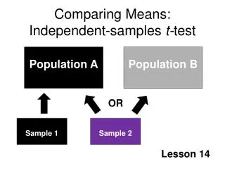
Research Designs • Independent Measures • Between-subjects • Making a comparison between two groups • Repeated Measures • Within-subjects • The two sets of data are obtained from the same sample
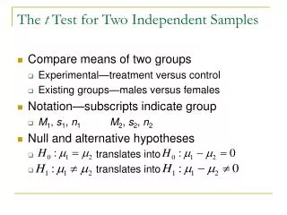
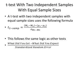
The t Test for Two Independent Samples • Compare means of two groups • Experimental—treatment versus control • Existing groups—males versus females • Notation—subscripts indicate group • M1, s1, n1 M2, s2, n2 • Null and alternative hypotheses • translates into • translates into
Same setup and logic • Compare what’s going on in data to what would be going if null hypothesis was true, taking into account variability from sample to sample • Larger the test statistic, less likely would get that by chance if the null hypothesis were true
Plugging in values • What’s going on in data = difference between means of each sample • What would be going on if null hypothesis were true = 0 (no difference between means) • Variability from sample to sample = standard error of the mean • But now we have two of them, since have two different samples
Computing two standard errors of the mean n1= n2 • Normally: sM = s2/n • Now with two samples: • S(M1-M2) = s12/n + s22/n
Computing two standard errors of the mean n1≠ n2 • First, need to deal with two sources of variance – variance in sample 1 and variance in sample 2 • Pool them together • Sp2 = SS total/df total • Referred to as pooled variance
Pooled Variance • Have two sources of df: • Sample 1 • Sample 2 • total df = dfsample 1 + dfsample 2 • df = df1 + df2 = (n1-1) + (n2-1) = n1 + n2 - 2
Pooled Variance • S2pooled = SS1 + SS2 df1 + df2
Computing two standard errors of the mean n1≠ n2 • Second, compute standard error of the mean • Normally: sM = √s2/n • With two samples to deal with:
t-test • t = sample mean diff – population mean diff estimated standard error
Hypothesis testing • Two-tailed • H0: µ1 = µ2, µ1 - µ2 = 0 • H1: µ1 ≠ µ2, µ1 - µ2 ≠ 0 • One-tailed • H0: µ1 ≥ µ2, µ1 - µ2 ≥ 0 • H1: µ1 < µ2, µ1 - µ2 < 0
Everything else is the same • As long as the calculated test statistic is more extreme than the critical t value, reject the null
Hypothesis testing • Determine α • Critical value of t • df = n1 + n2 - 2
Hypothesis Testing with t statistic • Step 1: State the hypotheses. • Step 2: Set and locate the critical region. • You will need to calculate the df to do this, and use the t distribution table. • Step 3: Graph rejection regions • Step 4: Collect sample data and compute t. • This will involve 3 calculations, given SS, n, , and M: • a) the sample variance (s2) • b) the estimated standard error (sM) • c) the t statistic
Hypothesis Testing with t statistic • Step 5: Make a decision • Need to compare tcalculated in Step 3 with tcriticalfound in the t table • If its two-tailed: • If tcalc > tCRIT (ignoring signs) Reject HO • If tcalc < tCRIT (ignoring signs) Fail to reject HO • If its one-tailed: You need to take the sign into consideration remembering to check back to the graph • Step 6: Interpret decision • Step 7: Find effect size
Example 1 • H0: µ1 = µ2, µ1 - µ2 = 0 • H1: µ1 ≠ µ2, µ1 - µ2 ≠ 0 • df = n1 + n2 - 2 =10 + 7 – 2 = 15 • =.05 • t(15) = 2.131
Example 1: t-test • t(15) = –2.325, p < .05 (precise p = 0.0345) • Reject H0
Example 2 • Mr. Fields owns construction companies in both Newport, Rhode Island and Miami, Florida • He feels that because of the warmer weather more of his employees in Miami take days off from work (presumably to party on South Beach). • In an interesting attempt to find out if this were true, he simply surveyed his employees as to how many days they frequented the beach in the last year. He believes that the data will reveal that the Miami workers spend more time at the beach than do the Newport workers. • On the next slide are the results of his survey • Sample 1 is Newport; Sample 2 is Miami
Example 2 • Step 1: State hypotheses • Sep2: Find tcritical
Example 2 • Step 4: Find tcalculated • Step 5: Make decision • Step 6: Interpret decision • Step 7: Determine effect size
Effect size • Cohen’s d = • Example 1 Cohen’s d • Example 2 Cohen’s d
Effect size • r2: amount of information you have about someone’s value on the dependent variable by knowing whether that person is from group 1 or group 2 • t2/t2+df
Effect size • Example 1: • r2 = t2/t2+df • r2 = ??? • Example 2: • r2 = t2/t2+df • r2 = ???
Assumptions • Random and independent samples • Normality • Homogeneity of variance • SPSS—test for equality of variances, unequal variances t test • t-test is robust
SPSS • Analyze • Compare Means • Independent-Samples T Test • Dependent variable(s)—Test Variable(s) • Independent variable—Grouping Variable • Define Groups • Cut point value • Output • Levene’s Test for Equality of Variances • t Tests • Equal variances assumed • Equal variances not assumed
Homogeneity of Variance • Calculating the pooled variance across the two samples assumes that it’s ok to combine them • Assumes that there is homogeneity of variance
Testing the Homogeneity of Variance • This, itself, is a hypothesis • Null hypothesis = no difference between variance of sample 1 and variance of sample 2 • When use SPSS to compute an independent samples t-test, this hypothesis is tested
Two t values to look at • SPSS then computes two t values, one in which the homogeneity of variance assumption is met, and the other in which it is not met • For the t in which the assumption is not met, the df will not be a whole number • Instead, df is lowered somewhat larger critical t more stringent test of differences between two groups
Telling the world • Same APA style as for one-sample t-tests: • t (df) = calculated t value, p information • Don’t forget to give the direction of significant differences! Give the mean and standard deviation of each group
Credits • http://myweb.liu.edu/~nfrye/psy801/ch10.ppt • http://faculty.plattsburgh.edu/alan.marks/Stat%20206/The%20t%20Test%20for%20Two%20Independent%20Samples.ppt