Download

1 / 48
490 likes | 675 Vues
Paired-Samples T-Test of Population Mean Differences. Key Points about Statistical Test Sample Homework Problem Solving the Problem with SPSS Logic for Paired-Samples T-Test of Population Mean Differences Power Analysis. Paired-samples T-Test: Purpose.

E N D
Paired-Samples T-Test of Population Mean Differences Key Points about Statistical Test Sample Homework Problem Solving the Problem with SPSS Logic for Paired-Samples T-Test of Population Mean Differences Power Analysis
Paired-samples T-Test: Purpose • Purpose: test whether or not the population mean represented by our sample has some specified value • Examples: • Social work students have higher GPA’s than other students • Social work students volunteer for more than 5 hours a week • UT social work students score higher on licensing exams than graduates of other programs • Social work students are getting younger every year
Paired-samples T-Test: Hypotheses • Hypotheses: • Null: population mean = specified value Versus • Research: population mean < specified value • Research: population mean ≠ specified value • Research: population mean > specified value • Decision: • Reject null hypothesis if pSPSS ≤ alpha (≠ relationship) • Reject null hypothesis if pSPSS÷2 ≤ alpha (< or > relationship)
Paired-samples T-Test: Assumptions and Requirements • Variable is interval level (ordinal with caution) • Variable is normally distributed • Acceptable degree of skewness and kurtosis or • Using the Central Limit Theorem
Paired-samples T-Test: Effect Size • Cohen’s d measures difference in means in standard deviation units. • Cohen’s d = population mean – specified value population standard deviation • Interpretation: • small: d = .20 to .50 • medium: d = .50 to .80 • large: d = .80 and higher
Paired-samples T-Test: APA Style • A paired-samples T-test is presented as follows: • t(75) = 2.11, p = .02 (one –tailed), d = .48 Degrees of freedom Value of statistic Significance of statistic Include if test is one-tailed Effect size if available
New dataset • These problems require a different type of data than what is available in GSS2000R. We need data where the same measure is administered multiple times. • The data set that we will used is called Omaha.sav, and can be downloaded from the course web site. • This data set contains a variety of attitude and functioning scales for a group of domestic violence victims from Omaha, taken one week, six months, and twelve months after the incident.
Coding scheme - 1 • To make the data amenable to the types of problems we will use it for, variables have been renamed and recoded. • There are four types of measures: • Variables on self esteem begin with the letters “se” • Variables on depression begin with the letters “dep” • Variables on locus of control being with “loc” • Variables on fears begin with the letters “fear”
Coding scheme - 2 • The time period for the measure is designated by the number following the initial letters: • 1 indicates 1 week after the incident, e.g. se1, loc1 • 6 indicates 6 months after the incident, e.g. se6, loc6 • 12 indicates 12 months after the incident, e.g. se12, loc6
Coding scheme - 3 • The specific content item is represented by an underscore followed by a number: • se1_1 is the item: Feel I'm a person of worth (1 week) • se6_4 is the item: Can do things as well as others (6 months)
Analyzing data in paired-sample tests • We will analyze relationships among various measures at different time periods, e.g. se1_1 versus se6_1, se1_1 versus se12_1, and se6_1 versus se12_1. • All of these items are rating scales, e.g. strongly disagree, disagree, agree, strongly agree. All have been recoded so that the most positive rating has the highest code number. • The variables are paired by questionnaire item, i.e. the respondent is the same for both questions.
Homework problems: Paired-Samples T-Test of Population Mean Differences This problem uses the data set OMAHA.Sav to compare the average difference between the variable "feeling of being a failure one week after the incident" [se1_3] and "feeling of being a failure six months after the incident" [se6_3]. Using an paired-samples t-test with an alpha of .05, is the following statement true, true with caution, false, or an incorrect application of a statistic? Victims of domestic violence significantly decreased their feeling of being a failure at six months after the incident (M = 1.64, SD = 0.66) over that at one week after the incident (M = 1.79, SD = 0.78) . • True • True with caution • False • Incorrect application of a statistic This is the general framework for the problems in the homework assignment on “Paired-Samples T-Test of Population Mean Differences.” The description is similar to findings one might state in a research article.
Homework problems: Paired-Samples T-Test - Data set, variables, and sample This problem uses the data set OMAHA.Sav to compare the average difference between the variable "feeling of being a failure one week after the incident" [se1_3] and "feeling of being a failure six months after the incident" [se6_3]. Using an paired-samples t-test with an alpha of .05, is the following statement true, true with caution, false, or an incorrect application of a statistic? Victims of domestic violence significantly decreased their feeling of being a failure at six months after the incident (M = 1.64, SD = 0.66) over that at one week after the incident (M = 1.79, SD = 0.78) . • True • True with caution • False • Incorrect application of a statistic • The first paragraph identifies: • The data set to use, e.g. OMAHA.Sav • The variable that will be compared in the analysis • Thealpha level to use for the hypothesis test
Homework problems: Paired-Samples T-Test - Specifications This problem uses the data set OMAHA.Sav to compare the average difference between the variable "feeling of being a failure one week after the incident" [se1_3] and "feeling of being a failure six months after the incident" [se6_3]. Using an paired-samples t-test with an alpha of .05, is the following statement true, true with caution, false, or an incorrect application of a statistic? Victims of domestic violence significantly decreased their feeling of being a failure at six months after the incident (M = 1.64, SD = 0.66) over that at one week after the incident (M = 1.79, SD = 0.78) . • True • True with caution • False • Incorrect application of a statistic • The second paragraph specifies: • The sample means and standard deviation for the variables being compared • The relationship for deriving the research hypothesis
Homework problems: Paired-SamplesT- Test - Choosing an answer The answer to a problem will be True if the t-test supports the finding in the problem statement. The answer to a problem will be True with caution if the t-test supports the finding in the problem statement, but the variable compared is ordinal level. This problem uses the data set OMAHA.Sav to compare the average difference between the variable "feeling of being a failure one week after the incident" [se1_3] and "feeling of being a failure six months after the incident" [se6_3]. Using an paired-samples t-test with an alpha of .05, is the following statement true, true with caution, false, or an incorrect application of a statistic? Victims of domestic violence significantly decreased their feeling of being a failure at six months after the incident (M = 1.64, SD = 0.66) over that at one week after the incident (M = 1.79, SD = 0.78) . • True • True with caution • False • Incorrect application of a statistic • The answer to a problem will Incorrect application of a statistic if • the t-test violates the level of measurement requirement, i.e. the variable is nominal level • the assumption of normality is violated and the central limit theorem cannot be applied The answer to a problem will be False if the t-test does not support the finding in the problem statement.
Solving the problem with SPSS:Level of measurement Statistical tests of means require that the dependent variable be interval level. "Feeling of being a failure one week after the incident" [se1_3] and “feeling of being a failure six months after the incident" [se6_3] are both ordinal level which violates the requirement for an interval dependent variable in the strictest interpretation of level of measurement. However, since the research literature often computes means for ordinal level data, especially scaled measures, we will follow the convention of applying interval level statistics to ordinal data. Since all analysts may not agree with this convention a caution is added to any true findings.
Solving the problem with SPSS: Creating a difference variable - 1 The Paired-Samples t-test uses the t-distribution for the probability of the test statistic, which tests whether the average of the differences between scores between the two variables is zero or not. The difference, which we will manually compute and test, is required to follow the normal distribution. We will generate descriptive statistics to evaluate normality. To create a variable for the differences between scores, select the Compute… command from the Transform menu.
Solving the problem with SPSS: Creating a difference variable - 2 Second, we subtract the variable in the earlier time period (one week) form the variable in the later time period (six months) to compute the value for the variable we are creating. First, type the name of the new variable in the Target Variable text box. Third, click on the OK button to complete the command.
Solving the problem with SPSS: Evaluating normality - 1 Select the Descriptive Statistics > Descriptives… command from the Analysis menu. The values for the difference variable are displayed in the data editor. We will generate descriptive statistics to evaluate normality.
Solving the problem with SPSS: Evaluating normality - 2 First, move the variable we will use in the t-test, difference, to the Variable(s) list box. Second, click on the Options… button to select the statistics we want.
Solving the problem with SPSS: Evaluating normality - 3 First, in addition to the statistics, SPSS has checked by default, mark the Kurtosis and Skewness check boxes on the Distribution panel. Second, click on the Continue button to close the dialog box.
Solving the problem with SPSS: Evaluating normality - 4 Click on the OK button to obtain the output.
Solving the problem with SPSS: Evaluating normality - 5 Differences between "feeling of being a failure one week after the incident" [se1_3] and "feeling of being a failure six months after the incident" [se6_3] did not satisfy the criteria for a normal distribution. The skewness of the distribution (-.325) was between -1.0 and +1.0, but the kurtosis of the distribution (1.287) fell outside the range from -1.0 to +1.0. However, since there were 438 valid cases, the assumption of normality was satisfied by the Central Limit Theorem which required that there be 30 or more cases.
Solving the problem with SPSS: The paired-samples t-test - 1 Having satisfied the level of measurement and assumption of normality, we now request the statistical test. Select Compare Means > Paired-Samples T Test… from the Analyze menu.
Solving the problem with SPSS: The paired-samples t-test - 2 Selecting the variables to compare in the paired-samples t-test is different than the method for most tests, and can be tricky. SPSS want us to select a pair of variables and then move the pair to the test list box. Click on the first variable in the pair, se1_3, to move it to the panel of Current Selections. Note: it does not matter which variable we select first. SPSS will change the order so that the variable which comes earlier in the data set will come first in the pair.
Solving the problem with SPSS: The paired-samples t-test - 3 While holding down the CTRL key on your keyboard, scroll down the list until the variable you want to choose is visible. Still holding down the CTRL key, click on the second variable in the pair, se6_3, to move it to the panel of Current Selections.
Solving the problem with SPSS: The paired-samples t-test - 4 With both variables in the Current Selections, click on the right arrow button to move the variables to the list box Paired Variables.
Solving the problem with SPSS: The paired-samples t-test - 5 Finally, click on the OK button to request the output. If you do not have the CTRL key held down before you scroll the list of variables and click on the second variable, you may find that the list is repositioned to display the wrong variables.
Solving the problem with SPSS: Answering the question - 1 The finding we are trying to verify is: Victims of domestic violence significantly decreased their feeling of being a failure at six months after the incident (M = 1.64, SD = 0.66) over that at one week after the incident (M = 1.79, SD = 0.78) . Our first task is to make certain the means and standard deviations are correctly cited. The mean and standard deviation at 1 week (M = 1.79, SD = 0.78) are correct. The mean and standard deviation at 6 months (M = 1.64, SD = 0.66) are correct.
Solving the problem with SPSS: Answering the question - 2 Our second task is to make certain the difference between the means is statistically significant at the alpha level stated in the problem, .05. The t-test supports the significance of the difference in means, t(437) = 3.930, p < .01 (one-tailed). The answer to the question is Truewith caution (the variables are ordinal scales). Since SPSS may change the order for the pair, the mean difference (e.g. .146) and the t-statistic may not have the correct sign. In this example, the average at six months was less than the average at 1 week, suggesting that the mean and t-statistic should have been negative. This is why I verify the direction of the test (increase or decrease) by examining the means of the samples, rather than relying on the sign of the mean difference. The feedback for homework problems will have the correct sign, though it may disagree with the SPSS output.
Logic for paired-samples t-test: Level of measurement and assumption of normality Measurement level of the pair of variables? Nominal/ Dichotomous Interval/ordinal Strictly speaking, the test requires interval level variable. We will allow ordinal level variables with a caution. Inappropriate application of a statistic Number of cases in both groups is at least 30? Skewness and Kurtosis between -1.0 and +1.0? No No Inappropriate application of a statistic Yes Yes
Logic for paired-samples t-test:Means and standard deviations correct Mean and standard deviation of both variables are correct? No Yes False
Logic for paired-samples t-test: Decision about null hypothesis One-tailed or two-tailed test? Two-tailed One-tailed Divide two-tailed significance by 2 Probability for t-test less than or equal to alpha? Yes No Add caution for ordinal variable. True False
Power Analysis: Paired-samples T-test Problem that was False This problem uses the data set OMAHA.Sav to compare the average difference between the variable "feeling like a person of worth one week after the incident" [se1_1] and "feeling like a person of worth six months after the incident" [se6_1]. Using an paired-samples t-test with an alpha of .05, is the following statement true, true with caution, false, or an incorrect application of a statistic? Victims of domestic violence significantly increased their feeling like a person of worth at six months after the incident (M = 3.50, SD = 0.59) over that at one week after the incident (M = 3.45, SD = 0.67) . 1 True 2 True with caution 3 False 4 Incorrect application of a statistic The answer to this problem was false because the probability for the t-test was .055 (one-tailed), greater than the alpha of 0.05. We can conduct a post-hoc power analysis to determine what number of cases would have been needed to have a better chance of finding a statistically significant difference.
Power Analysis: Statistical Results for Paired-samples T-test - 1 The answer to the problem was false because the one-tailed significance was p = .055 (.109 ÷ 2), less than the alpha of .05.
Power Analysis: Statistical Results for Paired-samples T-test - 2 We can calculate the effect size for the data for this problem, Cohen’s d, by dividing the Mean Difference (-.057) by the Std. Deviation (.744), which equals .08. Using Cohen’s criteria, a small effect size for difference in means would be .20, making the effect size for this data very small.
Access to SPSS’s SamplePower Program The UT license for SPSS does not include SamplePower, the SPSS program for power analysis. However, the program is available on the UT timesharing server. Information about access this program is available at this site.
Power Analysis for Paired-samples T-test - 1 In the SamplePower program on the ITS Timesharing Systems, select the New… command from the File menu.
Power Analysis for Paired-samples T-test - 2 First, select the Means tab to access the tests for means. Second, select the option button for Paired t-test that mean difference = 0. Third, click on the Ok button to enter the specific values for our problem.
Power Analysis for Paired-samples T-test - 3 The SD of the difference box may be disabled, identifiable by the gray text. To enable it, close the assistant dialog box.
Power Analysis for Paired-samples T-test – 4 I want to my entries to display three decimal places, instead of the default of 1, so I click on the Decimals displayed tool button.
Power Analysis for Paired-samples T-test – 5 First, click the up arrow button on the spinner for Decimals for data entry until 3 appears. Second, click on the OK button to close the dialog box.
Power Analysis for Paired-samples T-test - 6 SPSS sets the default test to a two-tailed test with an alpha of .05. Since our test was a one-tailed test with an alpha of .05, we click on the text specified as the SPSS default.
Power Analysis for Paired-samples T-test - 7 First, click on the 1 Tailed option on the Tails panel. Second, click on the Ok button to change the test specifications.
Power Analysis for Paired-samples T-test - 8 • We enter the values from the SPSS output from the Paired-samples t-test: • -.057 for Expected mean • .744 for Standard Deviation • 438 for the N of Cases When we have entered the values, click on the Compute button.
Power Analysis for Paired-samples T-test - 9 The power for the test was 48%, meaning that we had only a 50-50 chance of rejecting the null hypothesis. Although it is too late to redo the analysis, we can ask what size sample would we need if we wanted to redo the research and have an 80% chance of success.
Power Analysis for Paired-samples T-test - 10 To find the exact sample size needed, select Find N for power of 80% from the Tools menu.
Power Analysis for Paired-samples T-test - 11 To have a power of 0.80 with the very small effect size found in our data would have required a sample of over 1000 cases.