Download
1 / 38
430 likes | 768 Vues
Chapter 3. Propagation of Optical Beams in Fibers. 3.0 Introduction Optical fibers Optical communication - Minimal loss - Minimal spread - Minimal contamination by noise - High-data-rate In this chapter, - Optical guided modes in fibers

E N D
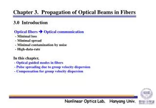
Chapter 3. Propagation of Optical Beams in Fibers 3.0 Introduction Optical fibers Optical communication - Minimal loss - Minimal spread - Minimal contamination by noise - High-data-rate In this chapter, - Optical guided modes in fibers - Pulse spreading due to group velocity dispersion - Compensation for group velocity dispersion
3.1 Wave Equations in Cylindrical Coordinates Refractive index profiles of most fibers are cylindrical symmetric Cylindrical coordinate system The wave equation for z component of the field vectors : where, and # Solve for first and then expressing in terms of Since we are concerned with the propagation along the waveguide, we assume that every component of the field vector has the same z- and t-dependence of exp[i(wt-bz)]
From Maxwell’s curl equations : We can solve for in terms of
Now, let’s determine (3.1-1) The solution takes the form : where, 1) where, : Bessel functions of the 1st and 2nd kind order of l 2) : Modified Bessel functions of the 1st and 2nd kind of order l where,
3.2 The Step-Index Circular Waveguide The field of confined modes : 1) (cladding region) : : evanescent (decay) wave * : virtually zero at * is not proper for the solution where, <Index profile of a step-index circular waveguide>
2) (core region) : : finite at * is not proper for the solution : propagating wave * where, * Necessary condition for confined modes to exist :
Boundary condition : tangential components of field are continuous at (3.2-10)
Condition for nontrivial solution to exist : (Report) (3.2-11) is to be determined for each l Amplitude ratios : [from (3.2-10) with determined eigenvalue b, Report] : the relative amount of Ez and Hz in a mode
Mode characteristics and Cutoff conditions (3.2-11) is quadratic in Two classes in solutions can be obtained, and designated as the EH and HE modes. (Hybrid modes) (3.2-11) By using the Bessel function relations : : EH modes (3.2-15) : Can be solved graphically : HE modes where,
Special case (l=0) 1) HE modes (3.2-15b) & (Report) From (3.2-10), Therefore, from (3.2-6)~(3.2-9), nonvanishing components are (TE modes) 2) EH modes (3.2-15a) & (Report) From (3.2-10), Therefore, from (3.2-6)~(3.2-9), nonvanishing components are (TM modes)
Graphical Solution for the confined TE modes (l=0) Roots of J0(ha)=0 should be real to achieve the exponential decay of the field in the cladding *
* If the max value of ha, V is smaller than the first root of J0(x), 2.405 => no TE mode * Cutoff value (a/l) for TE0m (or TM0m) waves : where, : mth zero of J0(x) * Asymtotic formula for higher zeros :
Special case (l=1) <EH modes> <HE modes> * HE mode does not have a cutoff. * All other HE1m, EH1m modes have cutoff value of a/l : * Asymptotic formula for higher zero :
The cutoff value for a/l (l>1) where, zlm is the mth root of
Propagation constant, b : (effective) mode index # : poorly confined : tightly confined # # V<2.405 Only the fundamental HE11 mode can propagate (single mode fiber)
3.3 Linearly Polarized Modes The exact expression for the hybrid modes (EHlm, HElm) are very complicated. If we assume n1-n2<<1 (reasonable in most fibers) a good approximation of the field components and mode condition can be obtained. (D. Gloge, 1971) Cartesian components of the field vectors may be used. <Wave equation for the Cartesian field components> 1) y-polarized waves (2.4-1), (3.1-2) & assume Ez<<Ey
After tedious calculations, (3.3-6)~(3.3-17), … (x, y) Expressions for the field components in core (r<a) Continuity condition : Expressions for the field components in cladding (r>a)
2) x-polarized waves (similar procedure to the case y-polarized waves) In core (r<a) Continuity condition Mode condition : simpler than (3.2-11) and/or In cladding (r>a) : This results also can be obtained from the y-polarized wave solution. x- and y-modes are degenerated.
Graphical Solution for the confined modes (l=0) <Possible distribution of LP11>
Mode cutoff value of a/l where, (3.3-27) Ex) l=0, Asymptotic formula for higher modes : Ref : Table 3-1Cutoff value of V for some low-order LP
Power flow and power density The time-averaged Poynting vector along the waveguide : (3.3-18), (2.3-19)
3.4 Optical Pulse Propagation and Pulse Spreading in Fibers One bit of information = digital pulse Limit ability to reduce the pulse width : Group velocity dispersion Group velocity dispersion Considering a Single mode / Gaussian pulse, temporal envelope at z=0 (input plane of fiber) : where, : transverse modal profile of the mode Fourier transformation : where,
Propagation delay factor for wave with the frequency of Let’s take complex expression and omit the (are not invloved in the analysis and can be restored when needed) Taylor series expansion : where, (3.4-5) : Field envelope
The pulse spreading is caused by the group velocity dispersion characterized by the parameter, (3.4-3)(3.4-5) :
# Pulse durationt at z (FWHM) # |aL|>>t0 (large distance) : initial pulse width If we use the definition of factor a, Practical Expression : where, : pulse transmission time through length L of the fiber
Group velocity dispersion 1) Material dispersion : n(w) depends on w 2) Waveguide dispersion : blm depends on w (& geometry of fiber) : modal dispersion i) ii) Single mode fiber, (3.4-18) waveguide dispersion material dispersion
From the uniform dielectric perturbation theory, : Fractions of power flowing in the core and cladding where, (3.4-18)
In weakly guiding fiber : n1~n2 Group velocity dispersion : ex) GeO2-doped silica : # depends on core diameter, n1, n2 control the waveguide shape
Group velocity dispersion & dispersion-flattened and dispersion-shifted fibers
Frequency chirping : modification of the optical frequency due to the dispersion (3.4-6) where, Total optical phase : Optical frequency :
3.5 Compensation for Group Velocity Dispersion (3.4-5) Fiber transfer function By convolution theorem, (1.6-2), : envelop impulse response of a fiber of length z
Compensation for pulse broadening 1) By optical fiber with opposite dispersion (a1L=-a2L)
2) By phase conjugation (a1L=a2L)
Where are (b) and (c) ?? Refer to the text <Experimental setup> <Eye diagram>
3.7 Attenuation in Silica Fibers Residual OH contamination of the glass 1.55 mm is favored for long-distance optical communication Recently, 400 Mb/s, 100 km @ 1.55 mm