Democratic Politics and Financial Markets
Democratic Politics and Financial Markets. William Bernhard University of Illinois bernhard@uiuc.edu David Leblang University of Colorado leblang@colorado.edu. What’s Hot in International Political Economy?. Economic Globalization Capital Mobility Trade Flows De-industrialization

Democratic Politics and Financial Markets
E N D
Presentation Transcript
Democratic Politics and Financial Markets William Bernhard University of Illinois bernhard@uiuc.edu David Leblang University of Colorado leblang@colorado.edu
What’s Hot in International Political Economy? • Economic Globalization • Capital Mobility • Trade Flows • De-industrialization • International Economic Institutions • Institutions: IMF, World Bank, WTO, EU • Exchange Rates, Currency Unions, Dollarization • International Financial Architecture • Domestic Political Change • Changes in Constituent Interests • Institutional Reform: Democratization, Electoral, Economic Policy
IPE and EITM: Two Great Tastes that Taste Great Together • Traditional Approaches in IPE • Developments since the 1980s • Concern with Domestic Politics • Enter Economics • Political Business Cycle • Partisanship Theory • Rational Expectations • Central Bank Independence • New Institutionalism • I.P.E. • Economic Foundations of Political Preferences • Political Sources of Economic Policy & Performance
Our Current Project • Connect International Capital Mobility and Institutional Reform • Democratic politics affects asset markets • Financial market behavior influences political processes • Combination of incentives create demands for institutional reform • Financial interests want less political uncertainty • Politicians want to insulate themselves from asset market volatility
Analytical Anchor: Financial Economics • Asset Markets • Exchange Rates • Spot • Forward • Bond • Government -- different maturities • Corporate -- usually constant maturity • Futures • Stocks • Distinguishing Features of Asset Markets • Prices fluctuate more than other markets (e.g., labor). • Assets have uncertain payments. Since they arise in the future, their present value is based on EXPECTATIONS of future payoffs. • Consequently, news and information arrival influences trading.
Efficient Markets Hypothesis • Assumptions of efficient market • Rational Actors • Symmetric Information (can be relaxed) • Zero Transactions Costs • Efficient Market Hypothesis • Deep markets quickly incorporate all information relevant to the price. • Implications • Prices move in a random walk • No unit root • Empirical Support for EMH
Critiques of the EMH • Empirical • Soundly rejected with forward exchange rates; bond markets (expectations hypothesis) • Use of high frequency data reveals non-stationarity, persistence, cointegration • Theoretical: Behavioral Finance • Asymmetric Information • Herding Behavior • Institutional Constraints
Political Information • Current work in IPE operates at a high level of institutional and temporal aggregation. • Think more carefully about political information and how it is processed • Political equilibrium and predictability • Updating • Empirical Strategy • Look at specific events • Temporal disaggregation
Organization of Project • Goal: Show Politics Affects Markets • Political Events and the Forward Exchange Rate Bias • Cabinet Formation and Market Behavior • Coalition Formation and Stock Markets • Coalition Bargaining and Government Bonds • The 2000 Presidential Elections and Overnight Trading • Goal: Show Markets Affect Politics • Polls and Pounds • Costs of Borrowing (Planned) • Incentives and Institutional Reform (Planned)
Coalition Formation • Cabinet Negotiations • Bargain over Policies (e.g., Schofield) • Bargain over Portfolios (e.g., Laver and Shepsle) • Laver and Shepsle • Cabinet Composition = f(Seats, Party Positions, Jurisdictional Structure) • Strong Party: A party is strong if it participates in every cabinet preferred by a majority to the cabinet in which that party forms a minority government. • At the very least, a strong party can veto certain alternative cabinets. • Strong parties tend to be at the median position. • Strong parties are more likely in party systems with fewer parties, fewer policy dimensions. • There can be at most one strong party.
The Winset Program • Winset Program • Requires Seats, Positions, Jurisdictions • Party Positions: Manifestos Data Set • Two Dimensions: Economic and Social • Three Dimensions: Economic, Social, Foreign • The program calculates • Whether a Strong Party exists • Simulations varying party position • No Strong Party: # of 1,000 Runs • 49 formations in 8 countries during the 1980s and 1990s
http://homepage.tinet.ie/~doylep/Winset/ws_index.htm The Winset Program
Two Dimensional Mapping Economic Dimension Pro-Market Pro-State Intervention Free Enterprise (401) Market Regulation (403) Incentives (402) minus Economic Planning (404) Protectionism Negative (407) Protectionism Positive (406) Economic Orthodoxy (414) Controlled Economy(412) Welfare State Limitation (505) Nationalization (413) Welfare State Expansion (504) Labor Groups: Positive (701) Social Dimension Numbers in Parentheses are Variable Numbers from Budge et. al 2001. Authoritarian Not Authoritarian Military: Positive (104) Anti-Imperialism (103) Freedom and Human Rights (201) Military: Negative (105) Constitutionalism: Positive (203) Peace (106) Political Authority (305) minus Internationalism: Negative (109) National Way of Life: Positive (601) Democracy (202) Traditional Morality: Positive (603) Education Expansion (506) Law and Order (605) Social Harmony (606) Construction of Policy Positions
Three Dimensional Mapping Economic Dimension Pro-Market Pro-State Intervention Free Enterprise (401) Market Regulation (403) Incentives (402) Economic Planning (404) Protectionism Negative (407) Protectionism Positive (406) Productivity (410) minus Demand Management (409) Economic Orthodoxy (414) Controlled Economy(412) Welfare State Limitation (505) Nationalization (413) Middle Class/Professional (704) Welfare State Expansion (504) Labor Groups: Positive (701) Cultural Dimension Authoritarian Not Authoritarian National Way of Life: Positive (601) Social Justice (503) Traditional Morality: Positive (603) Education Expansion (506) Law and Order (605) minus Traditional Morality: Negative (604) Social Harmony (606) Multiculturalism: Positive (607) Multiculturalism: Negative (608) Minority Groups (705) Non-Economic Groups (706) Foreign Policy Dimension Nationalist Internationalist Internationalism: Negative (109) minus Internationalism: Positive (107) European Community: Negative (110) European Community: Positive (108) Construction of Policy Positions
Event Period Estimation Period Campaign | Negotiation Step 1: Estimate Market Model for Estimation Window National Stock Returns= World Market, European Market Step 2: Using Parameter Estimates from Step 1, Calculate Residuals for Event Step 3: Average , test whether statistically different from zero. Calculating Average Abnormal Returns Event Study Methodology Estimation Period: 150 Days Event Window Campaign & Election Negotiation
Variable Campaign& Negotiation Negotiation Period 1 2 3 4 Constant -5.70 (3.281) 2.73 (1.52) -6.35 (3.05) 4.90* (1.57) Strong Party 7.313 (4.34) 9.08* (3.57) No Strong -0.008* (0.003) -0.011* (0.004) AAR for Campaign 0.482 (0.517) 0.527 (0.634) N=49 *p<.05 Robust standard errors in parentheses F 3.95 5.48 4.01 5.18 Prob F 0.0526 0.0474 0.0602 0.0361 Stock Market Experiment Regression Results
Conclusions and Extensions • Political predictability helps market actors adjust portfolios. • Extensions • Other political processes with predictable equilibrium. • More sophisticated models of asset returns.
Bargaining after the 1999 Austrian Election • October 3: Election • Early December: SPÖ-ÖVP Start Talks • January 19: SPÖ-ÖVP Agreement • January 21: SPÖ-ÖVP Collapses • January 24: ÖVP-FPÖ Negotiations • February 4: ÖVP-FPÖ Sworn-In
Bargaining after the 1996 New Zealand Elections • October 12: Election • October 21: National Party meets NZ First • October 23: Labour Party meets NZ First. Parties vow confidential negotiations. • October 29: Labour Party meets NZ First. • October 30: National Party meets NZ First. • November 19: NZ First says “Labour still in race” despite press speculation. • December 6: National Party caucus approves National-NZ First coalition. • December 7: Labour Party MPs approve Labour-NZ First coalition. • December 10: NZ First caucus chooses coalition with National Party.
Measuring the Dynamics of Coalition Bargaining • Content Analysis • 750 Articles from der Standard (Austria) • 141 Articles from The Post (NZ) • Coalition Under Discussion • Evaluation of Each Coalition: Likely, Neutral, Unlikely • Daily Frequency • Net Number of Likely Mentions • Likely Mentions – Unlikely Mentions • Coded as missing if coalition gets no mentions that day
where =mean of prior probability that the net number of likely mentions>0 =prior variance =data based probability that the net number of likely mentions>0 =data based variance N =sample size at time t. Updating the Probability of a Likely Mention • Prior beliefs condition impact of news. • For each coalition, calculate the updated probability that the net number of likely mentions will be positive:
Predicting Changes in Short-Term Interest Rates • Expectations Theory (Campbell and Shiller) • Change in Short-Term Rates = f(Spread Between Long-Term and Short-Term Rates) • Model • Vector Autoregression (VAR) • Short-Term: Overnight Rate • Spread: 10 year Rate – Overnight Rate • Two Lags • Political Variables as Exogenous • Sample • Austria: October 11, 1999-February 4, 2000 • New Zealand: October 19, 1996-December 19, 1996
∆rt St ∆rt St Net Mentions OVP-SPO -0.0003 (0.0007) -0.0003 (0.0008) Net Mentions OVP-FPO 0.0002 (0.0002) -0.0003 (0.0002) Net Mentions SPO-FPO 0.0010 (0.0020) -0.0005 (0.002) Posterior OVP-SPO -0.072* (0.031) 0.063* (0.033) Posterior OVP-FPO 0.079* (0.041) -0.077 (0.043) Cell entries are parameter estimates from a bivariate VAR that includes 2 lags of each dependent variable (not reported). Standard errors in parentheses. N=84 for both models. St is the spread between the long (10 year) and short (overnight) interest rate on Austrian government bonds. ∆rt is the change in the short rate. *p<0.05 Both models pass diagnostic tests for residual serial correlation, normality, heteroscedasticity and parameter constancy at the 0.05 level. Posterior SPO-FPO 0.312* (0.098) -0.356* (0.103) Bargaining and Bond Markets: VAR Results--Austria
∆rt St ∆rt St Net Mentions National-NZF -0.0006* (0.0002) 0.0001 (0.0003) Net Mentions Labour-NZF -0.0004 (0.0041) -0.0063 (0.0049) Posterior National-NZF -0.430* (0.133) 0.521* (0.152) Posterior Labour-NZF 0.115* (0.060) -0.140* (0.068) Cell entries are parameter estimates from a bivariate VAR that includes 2 lags of each dependent variable (not reported). Standard errors in parentheses. N=84 for both models. St is the spread between the long (10 year) and short (overnight) interest rate on New Zealand government bonds. ∆rt is the change in the short rate. *p<0.05 Both models pass diagnostic tests for residual serial correlation, normality, heteroscedasticity and parameter constancy at the 0.05 level. Bargaining and Bond Markets: VAR Results—New Zealand
Conclusions and Extensions • Implications: • Markets respond to publicly-available information. • Prior beliefs condition impact of events. • Extensions • Include other episodes of bargaining: Austria 2002-03. • Link bond and stock markets. • Bootstrapping VARs
Returns from S&P Statistical Issues of Financial Data I: Volatility Clustering
Returns from S&P Statistical Issues of Financial Data II: Kurtosis (Fat Tails)
Assessing the Predictability of Financial Data • OLS assumes errors are normally and independently distributed. Financial data often violate these assumptions. • Theoretical Concerns in Volatility/Predictability • Finance literature/risk premium, Black-Scholes pricing model • Economics literature/target zones • Political science literature/politics influence variability of asset prices • (e.g., Leblang and Bernhard; Freeman, Hays and Stix) • Key question: Are some events/periods/systems conducive to more/less volatility than others?
Basic ARCH (1) model: conditional variance of a shock at time t is a function of the squares of past shocks: where h is the variance and is a “shock,” “news,” or “error”. Since the conditional variance needs to be nonnegative, the conditions have to be met: . If 1 = 0, then the conditional variance is constant and is conditionally homoscedastic. The Autoregressive Conditional Heteroskedasticity (ARCH) Model • Autoregressive: it depends on its past • Conditional: variance depends on past information • Heteroskedasticity: non-constant variance • Invented by Engle (1982) to explain the volatility of inflation rates.
ARCH(p) models are difficult to estimate and decay very slowly. Therefore, Bollerslev (1986) developed the GARCH model. GARCH (1,1): The variance (ht) is a function of an intercept (), a shock from the prior period (), and the variance from last period (). Higher order GARCH models: The GARCH Model
A GARCH Model where = constant 2t-1 = GARCH t-1 = ARCH qt = Exog. variables
Sample GARCH Output GARCH (1,1) Model . arch dlsp, arch(1) garch(1) nolog ARCH family regression Sample: 4 to 223 Number of obs = 220 Wald chi2(.) = . Log likelihood = -366.1473 Prob > chi2 = . ----------------------------------------------------------------------------- | OPG dlsp | Coef. Std. Err. z P>|z| [95% Conf. Interval] -------------+---------------------------------------------------------------- dlsp | _cons | .0232815 .0826522 0.28 0.778 -.1387138 .1852768 -------------+---------------------------------------------------------------- ARCH | arch | L1 | .1652834 .045527 3.63 0.000 .0760521 .2545146 garch | L1 | .7815966 .0783583 9.97 0.000 .6280172 .935176 _cons | .1121176 .0913255 1.23 0.220 -.066877 .2911122 ------------------------------------------------------------------------------
Variations on the GARCH Model • Integrated GARCH (Engle and Bollerslev 1986). • Phenomenon is similar to integrated series in regular (ARMA-type) time-series. • Occurs when +=1. When this is the case it means that there is a unit root in the conditional variance; past shocks do not dissipate but persist for very long periods of time. • Fractionally Integrated GARCH (Baillie, Bollerslev and Mikkelsen (1996). • GARCH in Mean (Engle, Lilien and Robbins (1987). • Idea is that there is a direct relationship between risk and return of an asset. • In the mean equation, include some function of the conditional variance—usually the standard deviation. • This allows the mean of a series to depend, at least in part, on the conditional variance of the series .
Non-Linear GARCH Models • Non-Linear GARCH Models (dozens in last 20 years). • Linear GARCH models constrain prior shocks to have a symmetric affect on ht. • BUT there are theoretical reasons to believe that prior shocks will have an asymmetric impact on volatility. • Non-linear models allow for asymmetric shocks to volatility.
Conditional variance: where is the standardized residual and is the asymmetric component. The EGARCH Model • The Exponentional GARCH (EGARCH) model developed by Nelson (1991).
Brooks, Introductory Econometrics for Finance Enders, Applied Econometric Time Series Franses and van Dijk, Non-Linear Time Series Models in Empirical Finance Patterson, An Introduction to Applied Time Series Textbook References
The Immediate Financial Consequences of the 2000 Presidential Election
Overnight Trading on November 7 and 8, 2000 • Transactions (“tick”) data from the GLOBEX (overnight) market • 4:35pm EST – 8:59am EST. • Transactions aggregated to the minute. • Dependent Variable • Closing price (each minute) for NASDAQ 100 and S&P 500 Futures (maturity: 11/15/2000) • Calculated log differences and multiplied by 100
Political Information: Calling States • Calculate the probability of an electoral college victory for Gore. • Exploit the sampling uncertainty associated with polling data and calculate the probability, for each minute during the evening of November 7th, that Gore will win the electoral college. • Take the latest state level poll (vote share and sample size) and test the hypothesis: • Higher p-values indicate that the null cannot be rejected. Substantively it indicates the number of times, in repeated sampling, that Gore will win the popular vote in state i.
State Sample Size G% B% Gore/ (Bush+Gore) Prob Electoral Votes Time Called by CNN (est) Alaska 400 26 47 0.356 0.000 3 12:00am (B) Alabama 625 38 55 0.409 0.000 9 8:00pm (B) Arkansas 286 44 47 0.484 0.287 6 12:12am (B) Arizona 423 39 49 0.443 0.010 8 11:51pm (B) California 600 45 44 0.506 0.607 54 11:00pm (G) Colorado 400 38 47 0.447 0.017 8 11:41pm (B) Connecticut 447 48 32 0.600 1.000 8 8:00pm (G) Delaware 625 42 46 0.477 0.127 3 8:00pm (G) Florida 600 48 46 0.511 0.697 25 see below Georgia 512 37 53 0.411 0.000 13 7:59pm (B) Hawaii 261 50 31 0.617 1.000 4 11:00pm (G) Final State Polls