Polynomial Approximation
Polynomial Approximation. PSCI 702 October 05, 2005. What is a Polynomial?. Functions of the form: Polynomial of degree n, having n+1 terms. Will take n(n+1)n/2 multiplications and n additions. Can be re-written to take n additions and n multiplications. Factored form: N roots.


Polynomial Approximation
E N D
Presentation Transcript
Polynomial Approximation PSCI 702 October 05, 2005
What is a Polynomial? • Functions of the form: • Polynomial of degree n, having n+1 terms. • Will take n(n+1)n/2 multiplications and n additions. Can be re-written to take n additions and n multiplications.
Factored form: • N roots. • N+1 parameters. • Both real and complex roots. • No analytical solution for the polynomials of degree 5 or higher.
Iterative Methods • Searching with an initial guess the method finds the roots iteratively. • Construct a tangent to the curve at the initial guess and then extend this to the x-axis. • The new crossing point represent an improved value of the root.
Multiple Roots • A multiple root (double, triple, etc.) occurs where the function is tangent to the x axis two roots single root
Newton-Raphson Method Newton’s method - tangent line root x* xi+1 xi
Newton Raphson Method • Step 1: Start at the point (x1, f(x1)). • Step 2 : The intersection of the tangent of f(x) at this point and the x-axis. x2 = x1 - f(x1)/f `(x1) • Step 3: Examine if f(x2) = 0 or abs(x2 - x1) < tolerance, • Step 4: If yes, solution xr = x2 If not, x1 x2, repeat the iteration.
Newton-Raphson Method Examples of poor convergence
Secant Method • Use secant line instead of tangent line at f(xi)
Convergence not Guaranteed y = ln x
MATLAB Function: fzero • Bracketing methods – reliable but slow • Open methods – fast but possibly unreliable • MATLAB fzero– fast and reliable • fzero: find real root of an equation (not suitable for double root!) fzero(function, x0) fzero(function, [x0 x1])
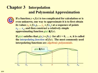
Interpolation Methods Interpolation uses the data to approximate a function, which will fit all of the data points. All of the data is used to approximate the values of the function inside the bounds of the data. All interpolation theory is based on polynomial approximation.
Lagrange Interpolation • The problem: find the (unique) polynomial f(x) of degree k-1 given a set of evaluation points {xi}i=1,k and a set of values {yi=f(xi)} Solution: for each i=1,...,k find a polynomial pi(x) that takes on the value yi at xi, and is zero for all other instances of x1, ...,xi-1,..xi+1,..xk
Cubic Lagrange Interpolation • p(x) = l1,4 f1 + l2,4 f2 + l3,4 f3 + l4,4 f4 • where • l1,4 = [ ( x - x2 ) ( x - x3 ) ( x - x4 ) ] / [ ( x1 - x2 ) ( x1 - x3 ) ( x1 - x4 ) ] • l2,4 = [ ( x - x1 ) ( x - x3 ) ( x - x4 ) ] / [ ( x2 - x1 ) ( x2 - x3 ) ( x2 - x4 ) ] • l3,4 = [ ( x - x1 ) ( x - x2 ) ( x - x4 ) ] / [ ( x3 - x1 ) ( x3 - x2 ) ( x3 - x4 ) ] • l4,4 = [ ( x - x1 ) ( x - x2 ) ( x - x3 ) ] / [ ( x4 - x1 ) ( x4 - x2 ) ( x4 - x3 ) ]
Cubic Lagrange Interpolation • Find the cubic polynomial whose graph contains the four successive points (0,1), (1,2), (2,0), and (3,-2). Setting x1 = 0, f1 = 1, x2 = 1, f2 = 2, x3 = 2, f3 = 0, and x4 = 3, f4 = -2, we can form the values of the ls • l1,4 = [ ( x - x2 ) ( x - x3 ) ( x - x4 ) ] / [ ( x1 - x2 ) ( x1 - x3 ) ( x1 - x4 ) ]= [ ( x - 1 ) ( x - 2 ) ( x - 3 ) ] / [ ( 0 - 1 ) ( 0 - 2 ) ( 0 - 3 ) ]= [ ( x - 1 ) ( x - 2 ) ( x - 3 ) ] / - 6 • l2,4 = [ ( x - x1 ) ( x - x3 ) ( x - x4 ) ] / [ ( x2 - x1 ) ( x2 - x3 ) ( x2 - x4 ) ]= [ ( x - 0 ) ( x - 2 ) ( x - 3 ) ] / [ ( 1 - 0 ) ( 1 - 2 ) ( 1 - 3 ) ]= [ x ( x - 2 ) ( x - 3 ) ] / 2 • l3,4 = [ ( x - x1 ) ( x - x2 ) ( x - x4 ) ] / [ ( x3 - x1 ) ( x3 - x2 ) ( x3 - x4 ) ]= [ ( x - 0 ) ( x - 1 ) ( x - 3 ) ] / [ ( 2 - 0 ) ( 2 - 1 ) ( 2 - 3 ) ]= [ x ( x - 1 ) ( x - 3 ) ] / - 2 • l4,4 = [ ( x - x1 ) ( x - x2 ) ( x - x3 ) ] / [ ( x4 - x1 ) ( x4 - x2 ) ( x4 - x3 ) ]= [ ( x - 0 ) ( x - 1 ) ( x - 2 ) ] / [ ( 3 - 0 ) ( 3 - 1 ) ( 3 - 2 ) ]= [ x ( x - 1 ) ( x - 2 ) ] / 6 .
Cubic Lagrange Interpolation • Inserting the values for the ls into Equation 2, we have • f(x) = l1,4 f1 + l2,4 f2 + l3,4 f3 + l4,4 f4= { [ ( x - 1 ) ( x - 2 ) ( x - 3 ) ] / - 6 } 1 + { [ x ( x - 2 ) ( x - 3 ) ] / 2 } 2 + { [ x ( x - 1 ) ( x - 3 ) ] / - 2 } 0 + { [ x ( x - 1 ) ( x - 2 ) ] / 6 } - 2 = (-1/6) [ ( x - 1 ) ( x - 2 ) ( x - 3 ) ] + [ x ( x - 2 ) ( x - 3 ) ] + (-1/3) [ x ( x - 1 ) ( x - 2 ) ] . • Multiplying out the terms and collecting yields the desired polynomial • f(x) = 0.5x3 - 3x2 + 3.5x + 1 .
Hermite Interpolation The Advantages • The segments of the piecewise Hermite polynomial have a continuous first derivative at support points (xis). • The shape of the function being interpolated is better matched, because the tangent of this function and tangent of Hermite polynomial agree at the support points
Cubic Spline Interpolation Hermite Polynomials produce a smooth interpolation, they have a disadvantage that the slope of the input function must be specified at each breakpoint. Cubic Splines interpolation use only the data points used to maintaining the desired smoothness of the function and is piecewise continuous.
Tangent vector p’(t) p(t) t
Significant values • p(0) : startpoint segment • p’(0) : tangent through startpoint • p(1) : endpoint segment • p’(1) : tangent through endpoint p’(0) p(1) t p’(1) p(0)
Rational Function Interpolation Polynomial are not always the best match of data. A rational function can be used to represent the steps. A rational function is a ratio of two polynomials. This is useful when you deal with fitting imaginary functions z=x + iy. The Bulirsch-Stoer algorithm creates a function where the numerator is of the same order as the denominator or 1 less.
Rational Function Interpolation The Rational Function interpolation are required for the location and function value need to be known. or
LegendrePolynomial The Legendre polynomials are a set of orthogonal functions, which can be used to represent a function as components of a function.
LegendrePolynomial These function are orthogonal over a range [-1, 1 ]. This range can be scaled to fit the function. The orthogonal functions are defined as:
Orthogonal Polynomials that covers the finite interval from -1 to 1 Legendre Polynomials
Orthogonal Polynomials that covers the semi finite interval from 0 to infinity. Laguerre Polynomials
Hermite polynomial • Orthogonal Polynomials that covers the infinite interval from -infinity to infinity.