Chapter 3 Interpolation and Polynomial Approximation

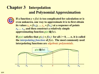
1. If a function y = f(x) is too complicated for calculation or is even unknown, one way to approximate it is to first obtain its values y0= f(x0), … yn= f(xn) at a sequence of points x0 … xn, and then construct a relatively simple approximating function g(x) f(x). If g(x) satisfies that g(xi) = f(xi) for all i = 0, … n, it is called the interpolating function of f(x). The most commonly used interpolating functions are …? x0 x1 x2 x x3 x4 Chapter 3Interpolation and Polynomial Approximation algebraic polynomials. g(x) f(x) 1/19

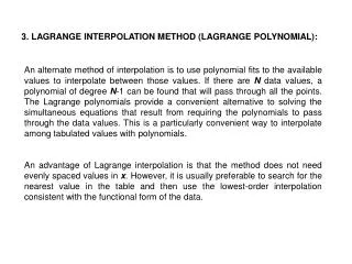
2. Chapter 3 Interpolation and Polynomial Approximation -- Interpolation and the Lagrange Polynomial Find a polynomial of degree n, Pn(x) = a0 + a1x + … + anxn, such that Pn(xi) = yi for all i = 0, …, n. - y y = + - 1 0 P ( x ) y ( x x ) - 1 0 0 x x 1 0 = y0+ y1 1  = ( x ) y L 1, i i = 0 i L1,0(x) L1,1(x) - - x x x x 0 1 - - x x x x 0 1 1 0  3.1 Interpolation and the Lagrange Polynomial Note: for any i j, we must have xi xj . Given x0, x1; y0,y1. Find P1(x) = a0 + a1x such that P1(x0) = y0 and P1(x1) = y1 . Lagrange Basis, satisfying L1,i(xj)=ij/* Kronecker Delta */ n = 1 P1(x) is the line function through the two given points ( x0, y0 ) and ( x1, y1) . 2/19

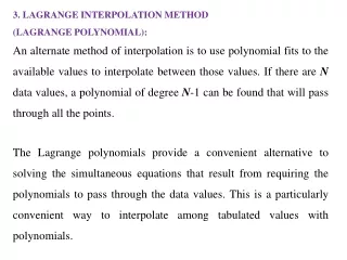
3. Chapter 3 Interpolation and Polynomial Approximation -- Interpolation and the Lagrange Polynomial The mathematician S. had to move to a new place. His wife didn't trust him very much, so when they stood down on the street with all their things, she asked him to watch their ten trunks, while she got a taxi. Some minutes later she returned. Said the husband: "I thought you said there were ten trunks, but I've only counted to nine!" The wife said: "No, they're TEN!" "But I have counted them: 0, 1, 2, ..." Find Ln,i(x) for i = 0, …, n such thatLn,i(xj)=ij . Then let . Hence Pn(xi) =yi . Each Ln,i has n roots x0 … xi … xn Ln,i(x) n  = - - - = - Ln,i(x) C ( x x )...( x x )...( x x ) C ( x x ) 0 i i n i j j  i n 1   y = 0 j = Ln,i Ln,i(x) = = P ( x ) ( x ) 1 C - n i i ( x x ) i j  i i = j 0 i n 1 The n-th Lagrange interpolating polynomial 3/19

4. Chapter 3 Interpolation and Polynomial Approximation -- Interpolation and the Lagrange Polynomial D(x) = Pn(x) – Qn(x) is a polynomial of degree Note: The interpolating polynomial is NOT unique unless its degree is constrained to be no greater than n. A counterexample is where p(x) can be a polynomial of any degree. Theorem: If x0, x1, …, xn are n + 1 distinct numbers and f is a function whose values are given at these numbers, then the n-th Lagrange interpolating polynomial is unique. Proof: If not… Then there exists two polynomials Pn(x) and Qn(x) both satisfying the interpolating conditions.  n Yet D(x) has distinct roots x0, x1, …, xn . n + 1 4/19

5. Chapter 3 Interpolation and Polynomial Approximation -- Interpolation and the Lagrange Polynomial Analyze the Remainder and f Cn + 1[a, b]. Suppose such that Consider the truncation error There exists such that n  = - R ( x ) K ( x ) ( x x ) n i = 0 i n  =  - g(t) Rn ( t ) K ( x ) ( t x ) i = 0 i g(x) has n+2 distinct roots x0 … xnx There exist + + + x - x - + = x - + ( 1 ) ( 1 ) ( 1 ) n n n R ( ) K ( x ) ( n 1 ) ! f ( ) P ( ) K ( x )( n 1 ) ! n x x n x + x ( 1 ) n f ( ) = x K ( x ) + ( n 1 ) ! There exists such that Rolle’s Theorem:If (x) is sufficiently smooth with (x0) = (x1) = 0, then there exists   (x0 , x1) such that  ’() = 0. Rn(x) has at least roots n+1 Fix anyx xi for all i = 0, …, n. Define the function g for t in [a, b] by In general, if (x0) = (x1) = (x2) = 0 5/19

6. Chapter 3 Interpolation and Polynomial Approximation -- Interpolation and the Lagrange Polynomial Note:  Since in most of the cases x cannot be determined, we obtain the upper bound of f (n+1) instead. That is, estimate an Mn+1 such that for all x(a,b) and take as the upper bound of the total error.  The interpolating polynomial is accurate for any polynomial function f with degree  n since f (n+1)(x)  0. A B C y y y 1 - 1 - 1 - 0.5 - 0.5 - 0.5 - x x x 0 1 2 3 4 5 6 0 1 2 3 4 5 6 0 1 2 3 4 5 6 - 0.5 - - 0.5 - - 0.5 - Quiz: Given xi = i +1, i = 0, 1, 2, 3, 4, 5. Which is the graph of L5, 2(x)?  6/19

7. Chapter 3 Interpolation and Polynomial Approximation -- Interpolation and the Lagrange Polynomial Example: Suppose a table is to be prepared for the function f(x) = ex for x in [0, 1]. Assume that each entry of the table is accurate up to 8 decimal places and the step size is h. What should h be for linear interpolation to give an absolute error of at most 10– 6 ? Solution: Suppose that [0, 1] is partitioned into n equal-spaced subintervals [x0, x1], [x1, x2], …, [xn–1 , xn], and x is in the interval [xk, xk+1]. Then the error estimation gives h 1.72  10–3 Simply take n = 1000 and h = 0.001. 7/19

8. Chapter 3 Interpolation and Polynomial Approximation -- Interpolation and the Lagrange Polynomial Example: Given Use the linear and the quadratic Lagrange polynomial of sin x to compute sin 50and then estimate the errors.  Use p 5 0.77614 Here   0 sin 50 P ( ) 1 18 and sin 50  0.76008,  Use Solution: First use x0, x1 and x1, x2 to compute the linear interpolations. In general, interpolation is better than extrapolation. sin 50 = 0.7660444… Error of extrapolation 0.01001 Error of interpolation 0.00596 8/19

9. Chapter 3 Interpolation and Polynomial Approximation -- Interpolation and the Lagrange Polynomial p 5 0.76543   0 sin 50 P ( ) 2 18 Now use x0, x1 and x2 to compute the quadratic interpolation. sin 50 = 0.7660444… Error of the quadratic interpolation 0.00061 Interpolation with higher degree usually obtain better results. The higher the better? Nooooooo…. 9/19

10. Chapter 3 Interpolation and Polynomial Approximation -- Interpolation and the Lagrange Polynomial When you start writing the program, you will find how easy it is to calculate the Lagrange polynomial. Oh yeah? What if I find the current interpolation not accurate enough? Right. Then all the Lagrange basis, Ln,i(x), will have to be re-calculated. Then you might want to take more interpolating points into account. Excellent point ! Let’s look at Neville’s Method… 10/19

11. Chapter 3 Interpolation and Polynomial Approximation -- Interpolation and the Lagrange Polynomial Definition: Let f be a function defined at x0, x1, …, xn, and suppose that m1, …, mk are k distinct integers with 0  mi n for each i. The Lagrange polynomial that agrees with f(x) at the k points denoted by Theorem: Let f be defined at x0, x1, …, xk, and let xi and xj be two distinct numbers in this set. Then describes the k-th Lagrange polynomial that interpolates f at the k+1 points x0, x1, …, xk . Proof: For any 0  r k and r i and j, the two interpolating polynomials on the numerator are equal to f(xr) at xr , so P(xr) = f(xr). The first polynomials on the numerator equals f(xi) at xi , while the second term is zero, so P(xi) = f(xi). Similarly P(xj) = f(xj). The k-th Lagrange polynomial that interpolates f at the k+1 points x0, x1, …, xk is unique. 11/19

12. Chapter 3 Interpolation and Polynomial Approximation -- Interpolation and the Lagrange Polynomial Neville’s Method x0 x1 x2 x3 x4 P0 P1 P2 P3 P4 P0,1 P1,2 P2,3 P3,4 P0,1,2 P1,2,3 P2,3,4 P0,1,2,3 P1,2,3,4 P0,1,2,3,4 HW: p.119 #5; p.120 #17 12/19

13. Chapter 3 Interpolation and Polynomial Approximation -- Divided Differences - f [ x , x , ... , x ] f [ x , ... , x , x ] = + 0 1 1 1 k k k f [ x , ... , x ] - + 0 1 k x x + 0 1 k - f [ x , ... , x , x ] f [ x , ... , x , x ] = - - + 0 1 0 1 1 k k k k - x x + 1 k k  3.2 Divided Differences The 1st divided difference of f w.r.t. xi and xj The 2nd divided difference of f w.r.t. xi , xj and xk The k+1st divided difference of f w.r.t. x0 … xk+1 13/19

14. Chapter 3 Interpolation and Polynomial Approximation -- Divided Differences As a matter of fact, where Warning: my head is exploding… What is the point of this formula? The value of f [ x0, …, xk ] is independent of the order of the numbers x0, …, xk . 14/19

15. Chapter 3 Interpolation and Polynomial Approximation -- Divided Differences 1 2 n1 + (x x0)  + … … + (x x0)…(x xn1)  1 2 n1 Newton’s Interpolation … … … … Nn(x) ai = f [ x0, …, xi ] Rn(x) 15/19

16. Chapter 3 Interpolation and Polynomial Approximation -- Divided Differences Note:  Since the n-th interpolating polynomial is unique, Nn(x)  Pn(x).  They must have the same truncation error. That is, The procedure is similar to Neville’s method. f (x0) f (x1) f (x2) … f (xn1) f (xn) f [x0, x1] f [x1, x2] … … … … f [xn1, xn] f [x0, x1 , x2] … … … … f [xn2, xn1, xn] f [x0, …, xn] f (xn+1) f [xn, xn+1] f [xn1, xn, xn+1] f [x1, …, xn+1] f [x0, …, xn+1] 16/19

17. Chapter 3 Interpolation and Polynomial Approximation -- Divided Differences If the points are equally spaced:  = - f f f + 1 i i i  = - - 1 k f f f - -  =   =  -  1 1 k k k f ( f ) f f i i i1 + 1 i i i i = - f f f - -    1 1 k k k - 1 i i i 其中 Formulae with Equal Spacing forward difference backward difference centered difference 17/19

18. Chapter 3 Interpolation and Polynomial Approximation -- Divided Differences Linearity: If f (x) is a polynomial of degree m , then is a polynomial of degree m – k and n n  D = - n j f ( 1 ) f + - k n k j j = 0 j where /* binomial coefficients */ n n  -  = - n n j f ( 1 ) f + - k k j n j = 0 j n n  = D j f f From Rn j + n k k D k f = 0 j = 0 f [ x , ... , x ] 0 k k k ! h D  k k f f x = ( ) k = 0 f ( ) n f [ x , x , ... , x ] - - 1 n n n k k h k k ! h Some important properties The values of the differences can be obtained from the function  And vice-versa  18/19

19. Chapter 3 Interpolation and Polynomial Approximation -- Divided Differences t n  Let , then = + =  k N ( x ) N ( x t h ) f ( x ) 0 0 n n k = 0 k Reverse the order of the points - t n  = + = -  k k Let , then N ( x ) N ( x t h ) ( 1 ) f ( x ) n n n n k = 0 k Newton’s formulae  Newton’s forward-difference formula HW: p.131 #5(a)(b); p.132 #13  Newton’s backward-difference formula 19/19