3. LAGRANGE INTERPOLATION METHOD (LAGRANGE POLYNOMIAL):
3. LAGRANGE INTERPOLATION METHOD (LAGRANGE POLYNOMIAL):.

3. LAGRANGE INTERPOLATION METHOD (LAGRANGE POLYNOMIAL):
E N D
Presentation Transcript
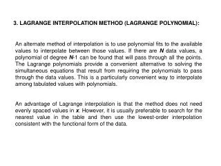
3. LAGRANGE INTERPOLATION METHOD (LAGRANGE POLYNOMIAL): An alternate method of interpolation is to use polynomial fits to the available values to interpolate between those values. If there are N data values, a polynomial of degree N-1 can be found that will pass through all the points. The Lagrange polynomials provide a convenient alternative to solving the simultaneous equations that result from requiring the polynomials to pass through the data values. This is a particularly convenient way to interpolate among tabulated values with polynomials. An advantage of Lagrange interpolation is that the method does not need evenly spaced values in x. However, it is usually preferable to search for the nearest value in the table and then use the lowest-order interpolation consistent with the functional form of the data.
li.txt 4 0,3 2,60 4,90 10,120 8 Sub lagri_Click () ' Change File li.txt for different problems fl = fl0 + "li.txt": Open fl For Input As 1 Input #1, nx: n=nx-1:ReDim xd(nx), f(nx) For k = 0 To n: Input #1, xd(k), f(k): Next k Input #1, x: Close #1 Call cls1: Print nx: Print For k = 0 To n: Print xd(k), f(k): Next k FX = 0 For k = 0 To n LKX = CDbl(1): LKXK = CDbl(1) For i = 0 To n If i = k Then 55 LKX = LKX * (x - xd(i)): LKXK = LKXK * (xd(k) - xd(i)) 55 Next i FX = FX + (LKX / LKXK) * f(k) Next k Print : Print " RESULT : ", x, FX End Sub
h Area of a single trapezoid = 4. NUMERICAL INTEGRATION: There are various numerical methods to calculate the definite integrals. The integral gives the area under the curve defined by the function f(x). We use the function values and increment value between to successive points on the x axis in order to calculate the integral. Trapezoidal Rule:
Simpson’s Rule: In Simpson’s rule, number of section n must be even! n=2*m n is always even number.
Example 4.1: Trapezoidal Rule gives: 0.743 Simpson’s Rule gives: 0.747 Sub trapezoidal_Click () ' CHANGE LINES 70 AND 75 FOR DIFFERENT PROBLEMS 70 a = 0: b = 1: n = 10 h = (b - a) / n j = 0: x = a For i = 0 To n c1 = 1: If i = 0 Or i = n Then c1 = .5 75 f = Exp(-x * x) j = j + h * c1 * f: x = x + h Next i Call cls1: Print : Print " RESULT : ", j End Sub
Sub simpson_Click () ' CHANGE LINES 80 AND 85 FOR DIFFERENT PROBLEMS 80 a = 0: b = 1: m = 4 n = 2 * m: h = (b - a) / n j = 0: x = a For i = 0 To n If i = 0 Or i = n Then c1 = 1: GoTo 85 If CInt(i / 2) = i / 2 Then c1 = 2: GoTo 85 c1 = 4 85 f = Exp(-x ^ 2) j = j + (h / 3) * c1 * f: x = x + h Next i Call cls1: Print : Print " RESULT : ", j End Sub