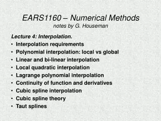
Chapter 14 Curve Fitting : Polynomial Interpolation

Chapter 14Curve Fitting : Polynomial Interpolation Gab Byung Chae

You’ve got a problem • Estimation of intermediate values between data points

14.1 Introduction to Interpolation

(2) MATLAB Function : polyfit and polyval Only one straight line that connects two points. Only one parabola connects a set of three points.

14.1.1 Determining polynomial coefficients • Interpolating polynomial of • solve • Ill-conditioned system (Vandermonde matrices)

4.1.2 MATLAB Functions >> format long >> T = [300 400 500]; >> density = [0.616 0.525 0.457]; >> p = polyfit(T, density,2) >> d = polyval(p,350)

14.2 Newton Interpolating polynomial

Graphical depiction of linear interpolation. The shaded areas indicate the similar triangles used to derive the Newton linear -interpolation formula [Eq. (14.5)]. Figure 14.2

FDD = finite divided difference The second FDD

Two linear interpolations to estimate ln 2. Note how the smaller interval provides a better estimate. Figure 14.3

Example 14.3 • Problem : f(x) = ln x • x1 = 1 f(x1) =0 • x2 = 4 f(x2) = 1.386294 • x3 = 6 f(x3) = 1.791759 • Solution : • b1 = 0 • b2 = (1.386294 – 0) /(4-1) = 0.4620981 • b3 = f2(x) = 0 + 0.4620981(x-1) – 0.0518731(x-1)(x-4)

The use of quadratic interpolation to estimate ln 2. The linear interpolation from x = 1 to 4 is also included for comparison. Figure 14.4

Newton Interpolation • Divided-difference table : Adding (3,14) and (4,22) <- a1 <- a2 <- a3

Graphical depiction of the recursive nature of finite divided differences. This representation is referred to as a divided difference table. Figure 14.5

Example 14.4 • Problem : f(x) = ln x • x1 = 1 f(x1) =0 • x2 = 4 f(x2) = 1.386294 • x3 = 6 f(x3) = 1.791759 • x4 = 5 f(x4) = 1.609438 f3(x) = b1 + b2(x-x1)+ b3(x-x1)(x-x2)+b4(x-x1)(x- x2)(x-x3)

Solution : • b1 = f(x1) = 0 • b2 = f[x2 , x1] = (1.386294 – 0) /(4-1) = 0.4620981 • f[x3,x2] = (1.791759 – 1.386294) /(6-4) = 0.2027326 • f[x4,x3] = (1.609438 – 1.791759) /(5-6) = 0.1823216 • b3 = f[x3 ,x2 ,x1] = (0.2027326 – 0.4620981) /(6-1) = -0.05187311 • f[x4 ,x3 ,x2] = (0.1823216 – 0.2027326) /(5-4) = -0.02041100 • b4 =f[x4 ,x3 ,x2,x1] = (-0.02041100 + 0.05187311) /(5-1) = 0.007865529

f3(x) = 0 + 0.4620981(x-1) - 0.05187311(x-1)(x-4) + 0.007865529(x-1)(x- 4)(x-6)

function yint = Newtint(x,y,xx) % yint = Newtint(x,y,xx): % Newton interpolation. Uses an (n - 1)-order Newton % interpolating polynomial based on n data points (x, y) % to determine a value of the dependent variable (yint) % at a given value of the independent variable, xx. % input: % x = independent variable % y = dependent variable % xx = value of independent variable at which % interpolation is calculated % output: % yint = interpolated value of dependent variable

% compute the finite divided differences in the form of a % difference table n = length(x); if length(y)~=n, error('x and y must be same length'); end b = zeros(n,n); % assign dependent variables to the first column of b. b(:,1) = y(:); % the (:) ensures that y is a column vector. for j = 2:n for i = 1:n-j+1 b(i,j) = (b(i+1,j-1)-b(i,j-1))/(x(i+j-1)-x(i)); end end % use the finite divided differences to interpolate xt = 1; yint = b(1,1); for j = 1:n-1 xt = xt*(xx-x(j)); yint = yint+b(1,j+1)*xt; end

14.3 Lagrange Interpolating polynomial The n-th order Lagrange interpolating polynomial weight coefficients The first order Lagrange interpolating polynomial

The second order Lagrange interpolating polynomial

Example 14.5 • Problem : Use a Lagrange interpolating polynomial of the first and second order to evaluate the density of unused motor oil at T = 15o C • x1 = 0 f(x1) = 3.85 • x2 = 20 f(x2) = 0.800 • x3 = 40 f(x3) = 0.212 • Solution : First-order at x=15: • f1(x)= Second-order : • f2(x)=

14.3.1 MATLAB M-file:Lagrange function yint = Lagrange(x,y,xx) % yint = Lagrange(x,y,xx): % Lagrange interpolation. Uses an (n - 1)-order Lagrange % interpolating polynomial based on n data points (x, y) % to determine a value of the dependent variable (yint) % at a given value of the independent variable, xx. % input: % x = independent variable % y = dependent variable % xx = value of independent variable at which the % interpolation is calculated % output: % yint = interpolated value of dependent variable

n = length(x); if length(y)~=n, error('x and y must be same length'); end s = 0; for i = 1:n product = y(i); for j = 1:n if i ~= j product = product*(xx-x(j))/(x(i)-x(j)); end end s = s+product; end yint = s;

14.4 Inverse Interpolation • (1,1) (3,3) (5,5) -> (?,2) • Polynomial interpolation • Determine (n-1)-th order polynomial p(x) • solve p(t) = 2 • Ex : (2, 0.5), (3,0.3333), and (4,0.25) • Find x so that f(x)=0.3 • f2 (x) = 0.041667x2 – 0.375x+1.08333 • Solve 0.3 = 0.041667x2 – 0.375x+1.08333 for x • x = 5.704158 or 3.295842

14.5.1 Extrapolation • Extrapolation is the process of estimating a value of f(x) that lies outside the range of the known base points.

Illustration of the possible divergence of an extrapolated prediction. The extrapolation is based on fitting a parabola through the first three known points. Figure 14.10

Example 14.6 • Problem : Fit a seventh-order polynomial to the first 8 points (1920 to 1990). Use it to compute the population in 2000 by extrapolationand compare your prediction with the actual result. • Solution : >> t = [1920 :10:1990]; >> pop = [106.46 123.08 132.12 152.27 180.67 205.05 227.23 249.46]; >> p = polyfit(t, pop, 7) Warning message ……

>> ts = (t-1955)/35; >> P = polyfit(ts, pop, 7); >> polyval(p, (2000-1955)/35) >>tt=linspace(1920,2000); >>pp=polyval(p, (tt-1955)/35); Plot(t,pop, ‘o’, tt, pp)

Use of a seventh-order polynomial to make a prediction of U.S. population in 2000 based on data from 1920 through 1990. Figure 14.11

14.5.2 Oscillations • Dangers of higher-order polynomial interpolation • Ex : Ringe’s function

Comparison of Runge’s function (dashed line) with a fourth-order polynomial fit to 5 points sampled from the function. Figure 14.12

Comparison of Runge’s function (dashed line) with a tenth-order polynomial fit to 11 points sampled from the function. Figure 14.13

Chapter 14 Curve Fitting : Polynomial Interpolation