Non-linear least square curve fitting method
Non-linear least square curve fitting method. Amey Modak, Yan zhu University of Washington. Introduction to least squares. Fitting a mathematical relationship to observations Approximate solution to over determined systems Least squares – the most commonly used method

Non-linear least square curve fitting method
E N D
Presentation Transcript
Non-linear least square curve fitting method Amey Modak, Yan zhu University of Washington
Introduction to least squares • Fitting a mathematical relationship to observations • Approximate solution to over determined systems • Least squares – the most commonly used method • Minimizes sum of residuals
Linear and Non-linear least squares • Depends on model function. • Linear least squares has residuals that are linear in all unknowns. • NLS have dependent on independent variable and the parameters. gradient equations do not have a closed solution. • This makes NLS an iterative method
Gauss-Newton method • Function • Sum of squares of Residual • Minimization: • have dependent on x and β. • This requires initial guess
Gauss-Newton Cond… • Improve parameter matrix iteratively • Linearize model after every iteration • Gradient equation: • Rearranging:
Problem definition • Material: copper • Dimensions = 1m X 1m X 0.01m • Thermal conductivity = 400 W/m-k • Rho = 8960 kg/m3 • Specific heat = 386 J/kg-k • Steffen Boltzmann constant = 5.670373e-8 • Convective heat coefficient = 1 • Ambient temperature = 300 K • Emissivity = 0.1
Gauss-Newton Solution • Model Function • Residual • Jacobians for each step:
Gauss-Newton Solution Cond… • Initial guess from Matlab lsqcurvfit [500; 4; 500; 0.1] • Use improved parameter matrix to iterate further • Continue iterations until (with prescribed error) • [528.17, 3.988, 469.16681, 0.07617905]
Conclusion • incredibly useful tool for analyzing sets of data • Converges faster if initial guesses are in the range • Robust method is useful to eliminate significant errors • Linear extrapolation for non-linear models gives significant errors • will not converge if the initial guesses are not in a suitable range

